El tradeoff bias-variance#
Compensación de sesgo y varianza
Versión b.1#
El notebook lo puedo modificar, esta versión es la b.1 a 17/11/2023 a las Caracas.
Aprendizaje Automático [UCV]#
Autor: Fernando Crema García
Contacto: fernando.cremagarcia@kuleuven.be; fernando.cremagarcia@esat.kuleuven.be
Preliminares#

All of Statistics: A concise course in Statistical Inference
Larry Wasserman

Un ejemplo con fotos#
Tomado de Bias Variance tradeoff Wikipedia

Alto bias, baja varianza

Alto bias, alta varianza

Bajo bias, baja variance

Bajo bias, alta variance
Breve repaso de probabilidades#
Leer [WASS] para profundizar. NO es requerido.
Vamos a hacer un ejemplo de la conexión entre estadística y probabilidades.
Estadístico: Dado un conjunto de datos un estadístico es una función aplicada a esos datos. Por ejemplo, el promedio muestral $\(\displaystyle \bar{x} = \frac{1}{n} \sum_{i=1}^n x_i\)$ es un estadístico (distinto de estadística, la ciencia).
Estimador: De alguna forma, buscamos conectar estadísticos muestrales de la “vida real” con estadísticos deconocidos (y teóricos) de la población de \(X\). Supongamos que existen parámetros poblacionales de \(X\) que llamaremos \(\theta\) que pertenecen a un conjunto \(𝛩\), es decir, \(\theta \in 𝛩\).
Dada una muestra aleatoria $\(x_1, x_2, ..., x_n \sim X \text{ muestreada de una distribución }X\)\( Un estimador \)\bar{\theta}\( es un **estadístico** usado para inferir \)\theta \in 𝛩\(. Por ejemplo, el **promedio muestral** \)\bar{x}\( es un estimador de la **media poblacional** \)\mu\(. Recordemos, \)\(\mu = \mathbb{E}(X)\)\( y que \)\( \mathbb{E}(X) = \begin{cases} \sum_{x} x P(X=x) & \text{ si } X \text{ es discreta} \\ \int x f(x) dx & \text{ si } X \text{ es continua} \\ \end{cases} \)$Bias (sesgo): El bias de un estimador \(\text{bias}(\theta, \bar{\theta}) \) está definido como $\(\text{bias}(\theta, \bar{\theta}) = \mathbb{E}[\bar{\theta}]-\theta\)\(. En el caso de \)\bar{x}\( y \)\mu\( tenemos \begin{aligned} \text{bias}(\mu, \bar{x}) & = \mu - \mathbb{E}\left[\frac{1}{n} \sum_{i=1}^n x_i\right] \\ & =\mu - \frac{1}{n} \sum_{i=1}^n \mathbb{E}\left(x_i\right) \\ & =\mu - \frac{1}{n} \sum_{i=1}^n \mu \\ & =\mu - \frac{1}{n}(n \mu) \\ & =\mu - \mu \\ \end{aligned} por lo que tenemos dos resultados \begin{aligned} E[x_i] & =\mu & \text{y además} \\ \text{bias}(\mu, \bar{x}) & = 0 \end{aligned} cuando \)\text{bias}(\theta, \bar{\theta}) = 0\( decimos que \)\bar{\theta}\( es un estimador **insesgado** de \)\theta$
La varianza poblacional de una variable aleatoria es la esperanza de la desviación cuadrática de su media poblacional y la denotamos \(\sigma\) o \(\mathbb{V}(X)\). Esto es: $\(\sigma = \mathbb{V}(X)=\mathbb{E}\left[(X-\bar{x})^2\right]\)\( La varianza muestral \)\(s^2 = \displaystyle \frac{1}{n} \sum_{i=1}^n (x_i - \mu)^2\)\( es fácil demostrar que \)\(\mathbb{E}(s^2) = \displaystyle \frac{n-1}{n} \sigma\)\( por lo que \)s^2\( NO es un **estimador insesgado** de \)\sigma\(. Es por esto que en la práctica, usamos la **varianza muestral insesgada** \)\(\bar{s}^2 = \displaystyle \frac{1}{n-1} \sum_{i=1}^n (x_i - \mu)^2\)$
Midiendo bias y varianza en OLS#
Hipótesis generales#
\(\mathbb{E}(\epsilon)=0\) : Los errores tienen media 0.
\(\operatorname{Var}(\epsilon)=\sigma^2 I\) : Los errores tienen varianza constante (homocedasticidad) y son independientes (no correlacionados).
\(X\) tiene rango full \(p\).
\(\hat{\beta}\) es insesgado#
Probemos que \(\hat{\beta}\) is insesgado. $\( \mathbb{E}(\hat{\beta})=\mathbb{E}\left(\left(X^T X\right)^{-1} X^T y\right) \)$
Sustituimos \(y=X \beta+\epsilon\) : $\( \begin{aligned} & \mathbb{E}(\hat{\beta})=\mathbb{E}\left(\left(X^T X\right)^{-1} X^T(X \beta+\epsilon)\right) \\ & \mathbb{E}(\hat{\beta})=\left(X^T X\right)^{-1} X^T \mathbb{E}(X \beta+\epsilon) \end{aligned} \)$
Como \(\mathbb{E}(\epsilon)=0\) : $\( \begin{gathered} \mathbb{E}(\hat{\beta})=\left(X^T X\right)^{-1} X^T X \beta \\ \mathbb{E}(\hat{\beta})=\beta \end{gathered} \)$
En consecuencia, \(\hat{\beta}\) es un estimador insesgado de \(\beta\).
Varianza de \(\hat{\beta}\)#
Encontremos la varianza de \(\hat{\beta}\). $\( \begin{gathered} \mathbb{Var}(\hat{\beta})=\mathbb{Var}\left(\left(X^T X\right)^{-1} X^T y\right) \\ \mathbb{Var}(\hat{\beta})=\left(X^T X\right)^{-1} X^T \mathbb{Var}(y) X\left(X^T X\right)^{-1} \end{gathered} \)$
Como \(y=X \beta+\epsilon\) y \(\mathbb{Var}(\epsilon)=\sigma^2 I\) : $\( \mathbb{Var}(y)=\mathbb{Var}(X \beta+\epsilon)=\sigma^2 I \)$
Entonces, $\( \begin{gathered} \mathbb{Var}(\hat{\beta})=\sigma^2\left(X^T X\right)^{-1} X^T X\left(X^T X\right)^{-1} \\ \mathbb{Var}(\hat{\beta})=\sigma^2\left(X^T X\right)^{-1} \end{gathered} \)$
Es entonces \(\hat{\beta}\) bueno?#
Sea \(\tilde{\beta}\) cualquier otro estimador lineal con varianza \(\mathbb{Var}(\tilde{\beta})\).
Podemos demostrar que \(\forall \tilde{\beta}\)
$\(
\operatorname{Var}(\tilde{\beta}) \geq \operatorname{Var}(\hat{\beta})
\)$
En consecuencia, el estimador OLS \(\hat{\beta}\) lo conocemos como el estimador “azul” BLUE: Best Linear Unbiased Estimator (BLUE) el mejor estimador insesgado lineal.
Qué rescatamos?#
\(\hat{\beta}\) es un estimador lineal de \(y\)
\(\hat{\beta}\) es insesgado
\(\hat{\beta}\) tiene varianza pero de los lineales, es el mejor.
El trade sesgo-varianza (bias-variance trade-off)#
Cómo podemos medir qué es más importante a la hora de tener sesgo y varianza?
Adaptado de [ISLP] página 32.
Regresemos a nuestro problema original.
Encontrar una función, denotada como \(f\), que mapee los datos de entrada \(X\) a los de salida \(y\). Es decir, $\(y= f(X) + \epsilon\)$
En general, no podemos conocer \(f\) y buscamos estimarla y buscar una \(\bar{f}\).
El bias (sesgo) de nuestra función será $\(\text{bias}(f, \bar{f}) = f-\mathbb{E}(\bar{f})\)\( y la varianza será \)\(\mathbb{E}\left[(f-\bar{f})^2\right]\)$
Imaginen ahora que queremos predecir para un \(x_0\). El error cuadrático medio sería:
Manipulando los términos, podemos llegar a una expresión que conecta (en el error cuadrático medio):
La varianza de \(\bar{f}(x_0)\)
El bias cuadrático de \(\bar{f}(x_0)\)
La varianza del ruido poblacional \(\epsilon\).
La expresión es:
Esta formula es la famosa base de la expresión “bias-variance tradeoff”
Regresemos a Ridge#
Ridge: Formulación lagrangeana#
\(h = 0\), \(\mathbf{L}=\mathbf{U}=\mathbf{0}\)
\(A = \mathbf{0}\), \(f(\mathbf{\hat{e}}) = {\frac{1}{2}\| \mathbf{\hat{e}} \|}^2_2\)
\(g(\mathbf{\beta}) = \lambda {\| \mathbf{\beta} \|}_2^2\).
Entonces, nuestro problema se convierte en:
Solución analítica#
Es insesgado?#
\begin{aligned} \widehat{\beta}^{\text {ridge }} & =\left(\mathbf{X}^{\mathrm{T}} \mathbf{X}+ \lambda \mathbf{I}\right)^{-1} \mathbf{X}^{\mathrm{T}} \mathbf{y} \ & =\left(\mathbf{X}^{\mathrm{T}} \mathbf{X}+ \lambda \mathbf{I}\right)^{-1}\left(\mathbf{X}^{\mathrm{T}} \mathbf{X}\right)\left(\mathbf{X}^{\mathrm{T}} \mathbf{X}\right)^{-1} \mathbf{X}^{\mathrm{T}} \mathbf{y} \ & =\left(\mathbf{X}^{\mathrm{T}} \mathbf{X}+ \lambda \mathbf{I}\right)^{-1}\left(\mathbf{X}^{\mathrm{T}} \mathbf{X}\right) \widehat{\beta}^{\text {ols }} \end{aligned}
Podemos analizar entonces
\(\widehat{\beta}^{\text {ridge }}\) es un estimador sesgado (dado que OLS es insesgado) para cualquier \(\lambda\) distinto de \(0\).
Si \(\lambda \rightarrow 0\), la solución de ridge tiende a OLS
Si \(\lambda \rightarrow \infty, \widehat{\beta}^{\text {ridge }} \rightarrow 0\)
Qué sucede con la varianza?#
Analicemos el caso extremo donde \(\mathbf{X}^{\mathrm{T}} \mathbf{X}= \mathbf{I}\),
\(\mathbf{X}\) es una matriz ortogonal con columnas estandarizadas y ortogonales.
Fíjense que cada \(\beta_j^{\text {ols }}\) es una proyección de \(\mathbf{y}\) sobre \(\mathbf{x}_j\), la \(j\)-ésima columna de \(X\).
Lo más importante: $\( \begin{aligned} \widehat{\beta}^{\text {ridge }} & =\left(\mathbf{X}^{\mathrm{T}} \mathbf{X}+n \lambda \mathbf{I}\right)^{-1}\left(\mathbf{X}^{\mathrm{T}} \mathbf{X}\right) \widehat{\beta}^{\text {ols }} \\ & =(\mathbf{I}+\lambda \mathbf{I})^{-1} \widehat{\beta}^{\text {ols }} \\ & =(1+\lambda)^{-1} \widehat{\beta}^{\text {ols }} \\ \Longrightarrow \beta_j^{\text {ridge }} & =\frac{1}{1+\lambda} \beta_j^{\text {ols }} \end{aligned} \)$
En consecuencia en este caso particular tanto el sesgo como la varianza las podemos expresar analíticamente como:
\(\operatorname{Bias}\left(\beta_j^{\text {ridge }}\right)=\frac{-\lambda}{1+\lambda} \beta_j^{\text {ols }}(\) distinto de 0 \()\)
\(\operatorname{Var}\left(\beta_j^{\text {ridge }}\right)=\frac{1}{(1+\lambda)^2} \operatorname{Var}\left(\beta_j^{\text {ols }}\right)\) (REDUCCIÓN DE OLS)
Desde el punto de vista estadístico, la función de complejidad básicamente añade sesgo a nuestros estimadores con la ventaja de reducir su varianza. Esto significa que se encuentran mejores estimadores para que podamos generalizar mejor para datos desconocidos.
Introducción a K-vecinos#
Uno de los modelos más simples de entender:
Parámetros: Entero \(K \in \mathbb{N}\)
Idea:: Si quiero predecir para un \(x_0\), encontrar los \(K\) puntos más cercanos a \(x_0\) y hacer un esquema de votación para cada \(c \in C\).
Importante:
El esquema de votación depende de nosotros.
Qué significa más cercano también.
Qué peculiaridad tiene este modelo?
from sklearn.datasets import load_iris
from sklearn.model_selection import train_test_split

iris = load_iris(as_frame=True)


X = iris.data[["sepal length (cm)", "sepal width (cm)"]]
y = iris.target
X_train, X_test, y_train, y_test = train_test_split(X, y, stratify=y, random_state=0)
---------------------------------------------------------------------------
ModuleNotFoundError                       Traceback (most recent call last)
Cell In[1], line 1
----> 1 from sklearn.datasets import load_iris
      2 from sklearn.model_selection import train_test_split
      4 iris = load_iris(as_frame=True)

ModuleNotFoundError: No module named 'sklearn'
iris = load_iris(as_frame=True)
iris
{'data':      sepal length (cm)  sepal width (cm)  petal length (cm)  petal width (cm)
 0                  5.1               3.5                1.4               0.2
 1                  4.9               3.0                1.4               0.2
 2                  4.7               3.2                1.3               0.2
 3                  4.6               3.1                1.5               0.2
 4                  5.0               3.6                1.4               0.2
 ..                 ...               ...                ...               ...
 145                6.7               3.0                5.2               2.3
 146                6.3               2.5                5.0               1.9
 147                6.5               3.0                5.2               2.0
 148                6.2               3.4                5.4               2.3
 149                5.9               3.0                5.1               1.8

 [150 rows x 4 columns],
 'target': 0      0
 1      0
 2      0
 3      0
 4      0
       ..
 145    2
 146    2
 147    2
 148    2
 149    2
 Name: target, Length: 150, dtype: int64,
 'frame':      sepal length (cm)  sepal width (cm)  petal length (cm)  petal width (cm)  \
 0                  5.1               3.5                1.4               0.2
 1                  4.9               3.0                1.4               0.2
 2                  4.7               3.2                1.3               0.2
 3                  4.6               3.1                1.5               0.2
 4                  5.0               3.6                1.4               0.2
 ..                 ...               ...                ...               ...
 145                6.7               3.0                5.2               2.3
 146                6.3               2.5                5.0               1.9
 147                6.5               3.0                5.2               2.0
 148                6.2               3.4                5.4               2.3
 149                5.9               3.0                5.1               1.8

      target
 0         0
 1         0
 2         0
 3         0
 4         0
 ..      ...
 145       2
 146       2
 147       2
 148       2
 149       2

 [150 rows x 5 columns],
 'target_names': array(['setosa', 'versicolor', 'virginica'], dtype='<U10'),
 'DESCR': '.. _iris_dataset:\n\nIris plants dataset\n--------------------\n\n**Data Set Characteristics:**\n\n    :Number of Instances: 150 (50 in each of three classes)\n    :Number of Attributes: 4 numeric, predictive attributes and the class\n    :Attribute Information:\n        - sepal length in cm\n        - sepal width in cm\n        - petal length in cm\n        - petal width in cm\n        - class:\n                - Iris-Setosa\n                - Iris-Versicolour\n                - Iris-Virginica\n                \n    :Summary Statistics:\n\n    ============== ==== ==== ======= ===== ====================\n                    Min  Max   Mean    SD   Class Correlation\n    ============== ==== ==== ======= ===== ====================\n    sepal length:   4.3  7.9   5.84   0.83    0.7826\n    sepal width:    2.0  4.4   3.05   0.43   -0.4194\n    petal length:   1.0  6.9   3.76   1.76    0.9490  (high!)\n    petal width:    0.1  2.5   1.20   0.76    0.9565  (high!)\n    ============== ==== ==== ======= ===== ====================\n\n    :Missing Attribute Values: None\n    :Class Distribution: 33.3% for each of 3 classes.\n    :Creator: R.A. Fisher\n    :Donor: Michael Marshall (MARSHALL%PLU@io.arc.nasa.gov)\n    :Date: July, 1988\n\nThe famous Iris database, first used by Sir R.A. Fisher. The dataset is taken\nfrom Fisher\'s paper. Note that it\'s the same as in R, but not as in the UCI\nMachine Learning Repository, which has two wrong data points.\n\nThis is perhaps the best known database to be found in the\npattern recognition literature.  Fisher\'s paper is a classic in the field and\nis referenced frequently to this day.  (See Duda & Hart, for example.)  The\ndata set contains 3 classes of 50 instances each, where each class refers to a\ntype of iris plant.  One class is linearly separable from the other 2; the\nlatter are NOT linearly separable from each other.\n\n.. topic:: References\n\n   - Fisher, R.A. "The use of multiple measurements in taxonomic problems"\n     Annual Eugenics, 7, Part II, 179-188 (1936); also in "Contributions to\n     Mathematical Statistics" (John Wiley, NY, 1950).\n   - Duda, R.O., & Hart, P.E. (1973) Pattern Classification and Scene Analysis.\n     (Q327.D83) John Wiley & Sons.  ISBN 0-471-22361-1.  See page 218.\n   - Dasarathy, B.V. (1980) "Nosing Around the Neighborhood: A New System\n     Structure and Classification Rule for Recognition in Partially Exposed\n     Environments".  IEEE Transactions on Pattern Analysis and Machine\n     Intelligence, Vol. PAMI-2, No. 1, 67-71.\n   - Gates, G.W. (1972) "The Reduced Nearest Neighbor Rule".  IEEE Transactions\n     on Information Theory, May 1972, 431-433.\n   - See also: 1988 MLC Proceedings, 54-64.  Cheeseman et al"s AUTOCLASS II\n     conceptual clustering system finds 3 classes in the data.\n   - Many, many more ...',
 'feature_names': ['sepal length (cm)',
  'sepal width (cm)',
  'petal length (cm)',
  'petal width (cm)'],
 'filename': 'iris.csv',
 'data_module': 'sklearn.datasets.data'}
X_train
| sepal length (cm) | sepal width (cm) | |
|---|---|---|
| 60 | 5.0 | 2.0 |
| 1 | 4.9 | 3.0 |
| 8 | 4.4 | 2.9 |
| 93 | 5.0 | 2.3 |
| 106 | 4.9 | 2.5 |
| ... | ... | ... |
| 66 | 5.6 | 3.0 |
| 29 | 4.7 | 3.2 |
| 130 | 7.4 | 2.8 |
| 141 | 6.9 | 3.1 |
| 111 | 6.4 | 2.7 |
112 rows × 2 columns
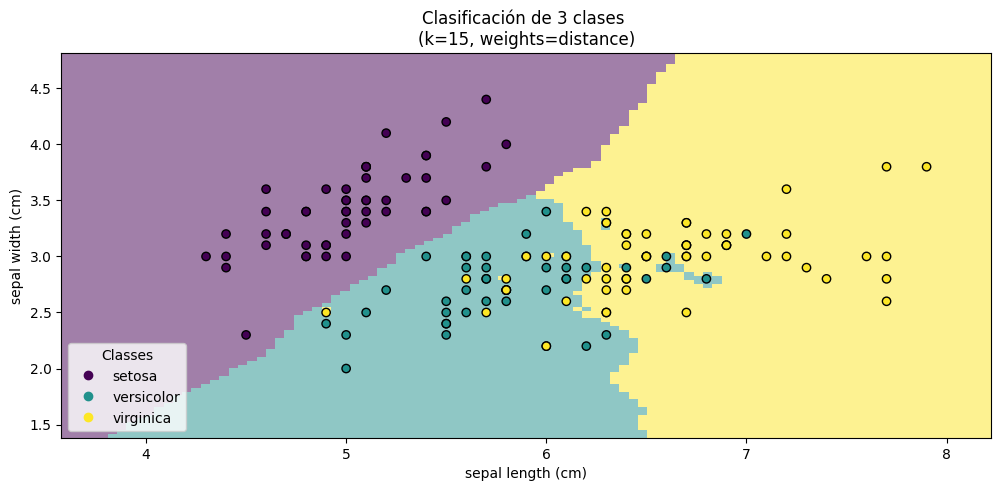
K=15
 from sklearn.neighbors import KNeighborsClassifier
 model = KNeighborsClassifier(n_neighbors=K)
import matplotlib.pyplot as plt

from sklearn.inspection import DecisionBoundaryDisplay

_, axs = plt.subplots(ncols=1, figsize=(12, 5))

model.set_params(weights="distance").fit(X_train, y_train)
disp = DecisionBoundaryDisplay.from_estimator(
    model,
    X_test,
    response_method="predict",
    plot_method="pcolormesh",
    xlabel=iris.feature_names[0],
    ylabel=iris.feature_names[1],
    shading="auto",
    alpha=0.5,
    ax=axs,
)
scatter = disp.ax_.scatter(X.iloc[:, 0], X.iloc[:, 1], c=y, edgecolors="k")
disp.ax_.legend(
    scatter.legend_elements()[0],
    iris.target_names,
    loc="lower left",
    title="Classes",
)
_ = disp.ax_.set_title(
    f"Clasificación de 3 clases \n(k={model.n_neighbors}, weights=distance)"
)
Con pipeline#
K = 1
from sklearn.neighbors import KNeighborsClassifier
from sklearn.pipeline import Pipeline
from sklearn.preprocessing import StandardScaler

clf = Pipeline(
    steps=[("scaler", StandardScaler()), ("knn", KNeighborsClassifier(n_neighbors=K))]
)
y_test
39     0
12     0
48     0
23     0
81     1
55     1
99     1
9      0
85     1
129    2
100    2
121    2
67     1
103    2
89     1
21     0
3      0
147    2
19     0
51     1
149    2
88     1
86     1
0      0
134    2
36     0
24     0
90     1
142    2
65     1
46     0
54     1
139    2
113    2
6      0
50     1
136    2
109    2
Name: target, dtype: int64
import matplotlib.pyplot as plt
from sklearn.inspection import DecisionBoundaryDisplay
_, axs = plt.subplots(ncols=2, figsize=(12, 5))
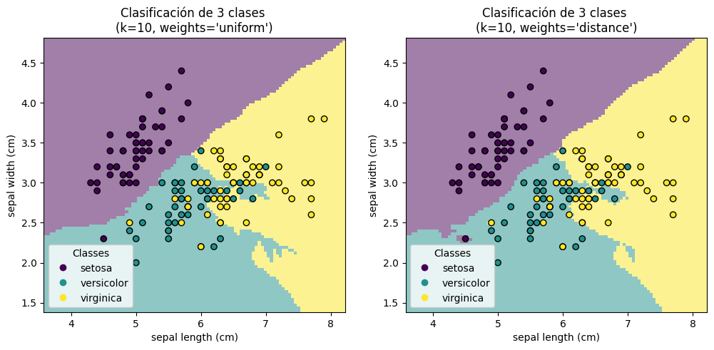
for ax, weights in zip(axs, ("uniform", "distance")):
clf.set_params(knn__weights=weights).fit(X_train, y_train)
disp = DecisionBoundaryDisplay.from_estimator(
clf,
X_test,
response_method="predict",
plot_method="pcolormesh",
xlabel=iris.feature_names[0],
ylabel=iris.feature_names[1],
shading="auto",
alpha=0.5,
ax=ax,
)
scatter = disp.ax_.scatter(X.iloc[:, 0], X.iloc[:, 1], c=y, edgecolors="k")
disp.ax_.legend(
scatter.legend_elements()[0],
iris.target_names,
loc="lower left",
title="Classes",
)
_ = disp.ax_.set_title(
f"Clasificación de 3 clases \n(k={clf[-1].n_neighbors}, weights={weights!r})"
)
plt.show()
from sklearn.metrics import accuracy_score, confusion_matrix
Matriz de confusión#
La entrada \(i,j\) de la matriz de confusión, \(M_{ij}\), representa el número de predicciones donde elementos de la clase \(i\) tuvo predicción \(j\).
Esto quiere decir que buscamos una matriz diagonal donde estén maximizadas las entradas \(i,i\) para toda clase \(i\)
confusion_matrix(y_test, clf.predict(X_test))
array([[13,  0,  0],
       [ 0,  7,  6],
       [ 0,  8,  4]])
Accuracy (Precisión)#
Métrica (estadístico) que responde a la pregunta: cuántas predicciones cuya clase inicial fue \(i\) tuvieron predicción \(i\). Esto quiere decir que el valor es la suma de la diagonal dividido entre el número de predicciones.
accuracy_score(y_test, clf.predict(X_test))
0.631578947368421
(13+7+4)/(13+7+4+8+6)
0.631578947368421
Conexión con variance-bias tradeoff#
Matemáticamente, buscamos: $\(\operatorname{Pr}\left(Y=c \mid X=x_0\right)=\frac{1}{K} \sum_{i \in \mathcal{V}_0} I\left(y_i=c\right) \)\( siendo \)\mathcal{V}_0\( la **vecindad** de \)x_0$
En [ESL] podemos encontrar una solución cerrada: $\(\mathbb{E}\left[(y-\bar{f}(x))^2 \mid X=x_0\right]=\left(f(x)-\frac{1}{k} \sum_{i=1}^k f\left(\mathcal{V}_i(x)\right)\right)^2+\frac{\sigma^2}{k}+\sigma^2\)$
Mientras \(k\) sea más pequeña, disminuye el bias y aumenta la varianza.
Para valores grandes de \(k\), aumenta el bias y disminuye la varianza.