07 Árboles de Decisión#
Versión v.1#
El notebook lo puedo modificar, esta versión es la b.1 a 10/07/2024 a las Caracas.
Aprendizaje Automático [UCV]#
Autor: Fernando Crema García
Contacto: fernando.cremagarcia@kuleuven.be; fernando.cremagarcia@esat.kuleuven.be
1. Intuición#
1.1 Funciones para graficar#
import matplotlib.pyplot as plt
import pandas as pd
from sklearn.datasets import load_iris
import warnings
warnings.filterwarnings('ignore')
---------------------------------------------------------------------------
ModuleNotFoundError                       Traceback (most recent call last)
Cell In[1], line 1
----> 1 import matplotlib.pyplot as plt
      2 import pandas as pd
      3 from sklearn.datasets import load_iris

ModuleNotFoundError: No module named 'matplotlib'
def plot_data_multiclass(X, y, idx=(0, 1), xi=None, yi=None):
  plt.figure(figsize=(10,10))
  plt.scatter(X[:, idx[0]], X[:, idx[1]], c=y, s=30, cmap=plt.cm.Paired)

  if xi is None or yi is None:
    plt.show()
    return 1

  plt.scatter(xi, yi, c=[3] if len(xi) == 1 else [3, 4], s=30)

  plt.scatter(
      xi,
      yi,
      s=100,
      linewidth=1,
      facecolors="none",
      edgecolors="k",
  )
  if len(xi) == 2:
    plt.plot(xi, yi, 'k-')
  plt.show()
1.2 Separando con hiperplanos simples#
Supongamos que solo vamos a separar de la forma \((j, t_i)\) con:
\(j\) el índice de alguna característica.
\(t_i\) un valor de la característica creando el intervalo \(x_j \leq t_i\)
X, y = load_iris(return_X_y=True)
type(X)
numpy.ndarray
X
y
array([0, 0, 0, 0, 0, 0, 0, 0, 0, 0, 0, 0, 0, 0, 0, 0, 0, 0, 0, 0, 0, 0,
       0, 0, 0, 0, 0, 0, 0, 0, 0, 0, 0, 0, 0, 0, 0, 0, 0, 0, 0, 0, 0, 0,
       0, 0, 0, 0, 0, 0, 1, 1, 1, 1, 1, 1, 1, 1, 1, 1, 1, 1, 1, 1, 1, 1,
       1, 1, 1, 1, 1, 1, 1, 1, 1, 1, 1, 1, 1, 1, 1, 1, 1, 1, 1, 1, 1, 1,
       1, 1, 1, 1, 1, 1, 1, 1, 1, 1, 1, 1, 2, 2, 2, 2, 2, 2, 2, 2, 2, 2,
       2, 2, 2, 2, 2, 2, 2, 2, 2, 2, 2, 2, 2, 2, 2, 2, 2, 2, 2, 2, 2, 2,
       2, 2, 2, 2, 2, 2, 2, 2, 2, 2, 2, 2, 2, 2, 2, 2, 2, 2])
Algunas veces, este criterio resulta poco útil
plot_data_multiclass(X, y)
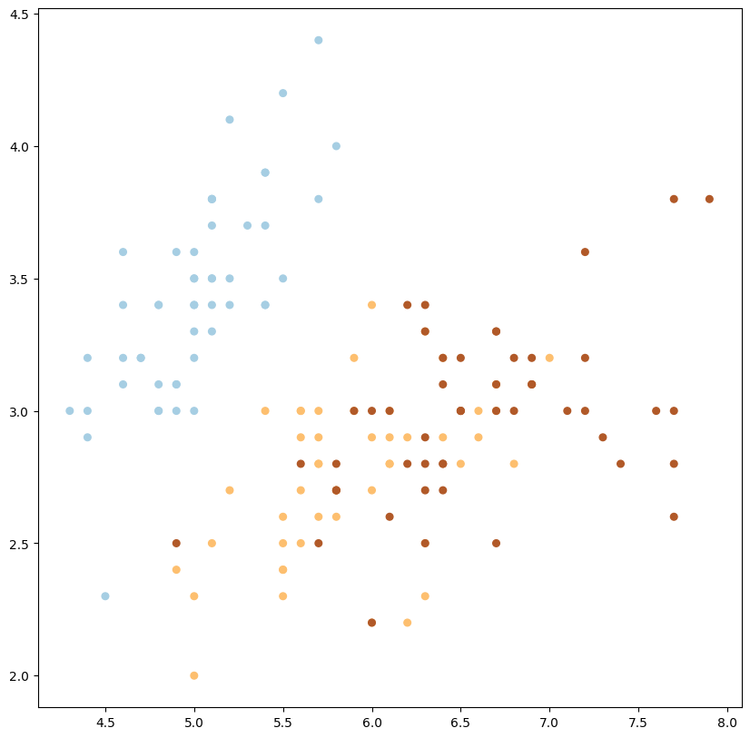
1
sin embargo, en algunos casos resulta útil
plot_data_multiclass(X, y, (0, 2))
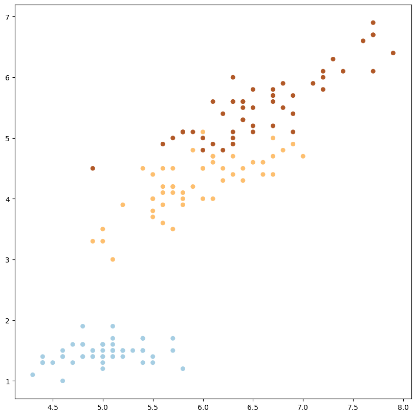
1
podemos modificar las dimensiones y podría funcionar también
plot_data_multiclass(X, y, (1, 2))
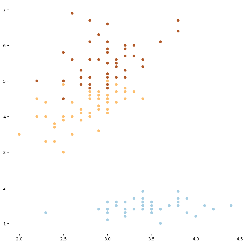
1
1.3 3D graph#
Veamos cómo se podría entender en tres dimensiones
1.3.1 Usando plotly#
import plotly.express as px
df = px.data.iris()
df
| sepal_length | sepal_width | petal_length | petal_width | species | species_id | |
|---|---|---|---|---|---|---|
| 0 | 5.1 | 3.5 | 1.4 | 0.2 | setosa | 1 |
| 1 | 4.9 | 3.0 | 1.4 | 0.2 | setosa | 1 |
| 2 | 4.7 | 3.2 | 1.3 | 0.2 | setosa | 1 |
| 3 | 4.6 | 3.1 | 1.5 | 0.2 | setosa | 1 |
| 4 | 5.0 | 3.6 | 1.4 | 0.2 | setosa | 1 |
| ... | ... | ... | ... | ... | ... | ... |
| 145 | 6.7 | 3.0 | 5.2 | 2.3 | virginica | 3 |
| 146 | 6.3 | 2.5 | 5.0 | 1.9 | virginica | 3 |
| 147 | 6.5 | 3.0 | 5.2 | 2.0 | virginica | 3 |
| 148 | 6.2 | 3.4 | 5.4 | 2.3 | virginica | 3 |
| 149 | 5.9 | 3.0 | 5.1 | 1.8 | virginica | 3 |
150 rows × 6 columns
fig = px.scatter(
    df, x='sepal_length', y='sepal_width',
    color='species',
    size = 'petal_length'
)

fig.show()
import plotly.express as px
df = px.data.iris()

fig = px.scatter_3d(
    df, x='sepal_length', y='sepal_width', z='petal_width',
    color='species',
    size = 'petal_length',

)

fig.show()
1.3.2 Usando scipy y plotly#
import scipy.io
import plotly.graph_objs as go
import numpy as np
iris = load_iris()
df = pd.DataFrame(
    data=np.c_[
        iris['data'],
        iris['target']
    ],
    columns= iris['feature_names'] + ['target']).astype({'target': int}).assign(
        species=lambda x: x['target'].map(dict(enumerate(iris['target_names'])))
    )
def md_graph(X, y, targets):
  # Get first y so we don't lose interpertrability later on
  classes = y.copy()

  x = X[targets[0]]
  y = X[targets[1]]
  z = X[targets[2]]
  fig = go.Figure(
      data=[
          go.Scatter3d(
              x=x,
              y=y,
              z=z,
              marker=dict(
                  size=6,
                  color=classes.values.reshape(150,),
                  opacity=0.8
              )
          )
      ]
  )

  fig.update_layout(
      scene=dict(
          xaxis_title=targets[0],
          yaxis_title=targets[1],
          zaxis_title=targets[2]),
      scx=1.5, y=3, z=0ene_camera=dict(
          up=dict(x=0, y=0, z=10),
          center=dict(x=0, y=0, z=0),
          eye=dict()
      )
  )
  fig.show()
df
| sepal length (cm) | sepal width (cm) | petal length (cm) | petal width (cm) | target | species | |
|---|---|---|---|---|---|---|
| 0 | 5.1 | 3.5 | 1.4 | 0.2 | 0 | setosa |
| 1 | 4.9 | 3.0 | 1.4 | 0.2 | 0 | setosa |
| 2 | 4.7 | 3.2 | 1.3 | 0.2 | 0 | setosa |
| 3 | 4.6 | 3.1 | 1.5 | 0.2 | 0 | setosa |
| 4 | 5.0 | 3.6 | 1.4 | 0.2 | 0 | setosa |
| ... | ... | ... | ... | ... | ... | ... |
| 145 | 6.7 | 3.0 | 5.2 | 2.3 | 2 | virginica |
| 146 | 6.3 | 2.5 | 5.0 | 1.9 | 2 | virginica |
| 147 | 6.5 | 3.0 | 5.2 | 2.0 | 2 | virginica |
| 148 | 6.2 | 3.4 | 5.4 | 2.3 | 2 | virginica |
| 149 | 5.9 | 3.0 | 5.1 | 1.8 | 2 | virginica |
150 rows × 6 columns
X = df.loc[:, ["sepal length (cm)"]]
X
| sepal length (cm) | |
|---|---|
| 0 | 5.1 |
| 1 | 4.9 |
| 2 | 4.7 |
| 3 | 4.6 |
| 4 | 5.0 |
| ... | ... |
| 145 | 6.7 |
| 146 | 6.3 |
| 147 | 6.5 |
| 148 | 6.2 |
| 149 | 5.9 |
150 rows × 1 columns
X_012, y_012 = df.iloc[:, [0, 1, 2]], df.loc[:, ["species"]]
md_graph(X=X_012, y=y_012, targets=["sepal length (cm)", "sepal width (cm)", "petal length (cm)"] )
---------------------------------------------------------------------------
ValueError                                Traceback (most recent call last)
<ipython-input-168-4c4f56603923> in <cell line: 1>()
----> 1 md_graph(X=X_012, y=y_012, targets=["sepal length (cm)", "sepal width (cm)", "petal length (cm)"] )

<ipython-input-160-2f942e4ec992> in md_graph(X, y, targets)
      8   fig = go.Figure(
      9       data=[
---> 10           go.Scatter3d(
     11               x=x,
     12               y=y,

/usr/local/lib/python3.10/dist-packages/plotly/graph_objs/_scatter3d.py in __init__(self, arg, connectgaps, customdata, customdatasrc, error_x, error_y, error_z, hoverinfo, hoverinfosrc, hoverlabel, hovertemplate, hovertemplatesrc, hovertext, hovertextsrc, ids, idssrc, legend, legendgroup, legendgrouptitle, legendrank, legendwidth, line, marker, meta, metasrc, mode, name, opacity, projection, scene, showlegend, stream, surfaceaxis, surfacecolor, text, textfont, textposition, textpositionsrc, textsrc, texttemplate, texttemplatesrc, uid, uirevision, visible, x, xcalendar, xhoverformat, xsrc, y, ycalendar, yhoverformat, ysrc, z, zcalendar, zhoverformat, zsrc, **kwargs)
   2668         _v = marker if marker is not None else _v
   2669         if _v is not None:
-> 2670             self["marker"] = _v
   2671         _v = arg.pop("meta", None)
   2672         _v = meta if meta is not None else _v

/usr/local/lib/python3.10/dist-packages/plotly/basedatatypes.py in __setitem__(self, prop, value)
   4863                 # ### Handle compound property ###
   4864                 if isinstance(validator, CompoundValidator):
-> 4865                     self._set_compound_prop(prop, value)
   4866
   4867                 # ### Handle compound array property ###

/usr/local/lib/python3.10/dist-packages/plotly/basedatatypes.py in _set_compound_prop(self, prop, val)
   5274         # ------------
   5275         validator = self._get_validator(prop)
-> 5276         val = validator.validate_coerce(val, skip_invalid=self._skip_invalid)
   5277
   5278         # Save deep copies of current and new states

/usr/local/lib/python3.10/dist-packages/_plotly_utils/basevalidators.py in validate_coerce(self, v, skip_invalid, _validate)
   2473
   2474         elif isinstance(v, dict):
-> 2475             v = self.data_class(v, skip_invalid=skip_invalid, _validate=_validate)
   2476
   2477         elif isinstance(v, self.data_class):

/usr/local/lib/python3.10/dist-packages/plotly/graph_objs/scatter3d/_marker.py in __init__(self, arg, autocolorscale, cauto, cmax, cmid, cmin, color, coloraxis, colorbar, colorscale, colorsrc, line, opacity, reversescale, showscale, size, sizemin, sizemode, sizeref, sizesrc, symbol, symbolsrc, **kwargs)
   1265         _v = color if color is not None else _v
   1266         if _v is not None:
-> 1267             self["color"] = _v
   1268         _v = arg.pop("coloraxis", None)
   1269         _v = coloraxis if coloraxis is not None else _v

/usr/local/lib/python3.10/dist-packages/plotly/basedatatypes.py in __setitem__(self, prop, value)
   4871                 # ### Handle simple property ###
   4872                 else:
-> 4873                     self._set_prop(prop, value)
   4874             else:
   4875                 # Make sure properties dict is initialized

/usr/local/lib/python3.10/dist-packages/plotly/basedatatypes.py in _set_prop(self, prop, val)
   5215                 return
   5216             else:
-> 5217                 raise err
   5218
   5219         # val is None

/usr/local/lib/python3.10/dist-packages/plotly/basedatatypes.py in _set_prop(self, prop, val)
   5210
   5211         try:
-> 5212             val = validator.validate_coerce(val)
   5213         except ValueError as err:
   5214             if self._skip_invalid:

/usr/local/lib/python3.10/dist-packages/_plotly_utils/basevalidators.py in validate_coerce(self, v, should_raise)
   1352
   1353                 if invalid_els and should_raise:
-> 1354                     self.raise_invalid_elements(invalid_els)
   1355
   1356                 # ### Check that elements have valid colors types ###

/usr/local/lib/python3.10/dist-packages/_plotly_utils/basevalidators.py in raise_invalid_elements(self, invalid_els)
    301     def raise_invalid_elements(self, invalid_els):
    302         if invalid_els:
--> 303             raise ValueError(
    304                 """
    305     Invalid element(s) received for the '{name}' property of {pname}

ValueError:
    Invalid element(s) received for the 'color' property of scatter3d.marker
        Invalid elements include: ['setosa', 'setosa', 'setosa', 'setosa', 'setosa', 'setosa', 'setosa', 'setosa', 'setosa', 'setosa']

    The 'color' property is a color and may be specified as:
      - A hex string (e.g. '#ff0000')
      - An rgb/rgba string (e.g. 'rgb(255,0,0)')
      - An hsl/hsla string (e.g. 'hsl(0,100%,50%)')
      - An hsv/hsva string (e.g. 'hsv(0,100%,100%)')
      - A named CSS color:
            aliceblue, antiquewhite, aqua, aquamarine, azure,
            beige, bisque, black, blanchedalmond, blue,
            blueviolet, brown, burlywood, cadetblue,
            chartreuse, chocolate, coral, cornflowerblue,
            cornsilk, crimson, cyan, darkblue, darkcyan,
            darkgoldenrod, darkgray, darkgrey, darkgreen,
            darkkhaki, darkmagenta, darkolivegreen, darkorange,
            darkorchid, darkred, darksalmon, darkseagreen,
            darkslateblue, darkslategray, darkslategrey,
            darkturquoise, darkviolet, deeppink, deepskyblue,
            dimgray, dimgrey, dodgerblue, firebrick,
            floralwhite, forestgreen, fuchsia, gainsboro,
            ghostwhite, gold, goldenrod, gray, grey, green,
            greenyellow, honeydew, hotpink, indianred, indigo,
            ivory, khaki, lavender, lavenderblush, lawngreen,
            lemonchiffon, lightblue, lightcoral, lightcyan,
            lightgoldenrodyellow, lightgray, lightgrey,
            lightgreen, lightpink, lightsalmon, lightseagreen,
            lightskyblue, lightslategray, lightslategrey,
            lightsteelblue, lightyellow, lime, limegreen,
            linen, magenta, maroon, mediumaquamarine,
            mediumblue, mediumorchid, mediumpurple,
            mediumseagreen, mediumslateblue, mediumspringgreen,
            mediumturquoise, mediumvioletred, midnightblue,
            mintcream, mistyrose, moccasin, navajowhite, navy,
            oldlace, olive, olivedrab, orange, orangered,
            orchid, palegoldenrod, palegreen, paleturquoise,
            palevioletred, papayawhip, peachpuff, peru, pink,
            plum, powderblue, purple, red, rosybrown,
            royalblue, rebeccapurple, saddlebrown, salmon,
            sandybrown, seagreen, seashell, sienna, silver,
            skyblue, slateblue, slategray, slategrey, snow,
            springgreen, steelblue, tan, teal, thistle, tomato,
            turquoise, violet, wheat, white, whitesmoke,
            yellow, yellowgreen
      - A number that will be interpreted as a color
        according to scatter3d.marker.colorscale
      - A list or array of any of the above
1.3.2.a Solved#
X_012, y_012 = df.iloc[:, [0, 1, 2]], df.loc[:, ["target"]]
X_012["sepal length (cm)"]
0      5.1
1      4.9
2      4.7
3      4.6
4      5.0
      ...
145    6.7
146    6.3
147    6.5
148    6.2
149    5.9
Name: sepal length (cm), Length: 150, dtype: float64
md_graph(X=X_012, y=y_012, targets=["sepal length (cm)", "sepal width (cm)", "petal length (cm)"] )
2. Formalizando matemáticamente#
Vayamos a la definición de árboles de clasificación en scikit
Dados los vectores de entrenamiento \(x_s \in \mathbb{R}^p, \mathrm{i}=1, \ldots\), n y un vector de clases \(y \in \mathbb{R}^n\), un árbol de decisión divide recursivamente el espacio de características de modo que las muestras con las mismas etiquetas o valores objetivo similares se agrupen juntas.
2.1 Los candidatos#
Sean los datos en el nodo \(i\) representados por \(Q_i\) con \(n_i\) muestras.
Para cada división candidata \(\theta=\left(j, t_i\right)\) que consta de una característica \(j\) y un umbral \(t_i\), divide el nodo en
\(Q_i^{\text {izq }}(\theta)\) y
\(Q_i^{\text {right }}(\theta)\)
Donde

2.1 Midiendo la calidad de un candidato#
El problema es que podemos tener infinitos cortes \(\theta\) por lo que tenemos que tener un método para definiir qué tan bueno es dentro de un conjunto de opciones y escoger el mejor.
La calidad de una división candidata del nodo \(i\) se calcula utilizando una función de impureza o función de pérdida \(H()\), cuya elección depende de la tarea que se resuelve (clasificación o regresión).
Fíjense como \(H\) la definen sin parámetros porque pueden variar dependiendo de H
Seleccionar el mejor \(\theta\) que minimice la impureza. $\( \theta^*=\operatorname{argmin}_\theta G\left(Q_i, \theta\right) \)$
Fíjense como \(Q_i\) permanece estático porque buscamos es el mejor \(\theta\) para ese nodo \(i\)
De manera recursiva, ejecutamos ahora para los subconjuntos \(Q_i^{\text{izq}}\left(\theta^*\right)\) y \(Q_i^{\text{der}}\left(\theta^*\right)\) hasta el máximo permitido
2.2 Criterios de parada#
Se alcanza la profundidad, \(n_i<\min _{\text {samples }}\) o \(n_i=1\).
2.3 Criterios para clasificación#
Si el objetivo es hacer clasificación sobre las clases $\(n_c \in \{0,1, \ldots, \mathrm{N}-1\}\)\(, para el nodo \)i\(, tenemos \)\( p_{i n_c}=\frac{1}{n_i} \sum_{y \in Q_i} I(y=n_c) \)\( la proporción de la clase \)\mathrm{n_c}\( en el nodo \)i\(. Si \)i\( es un nodo terminal, predict_proba para la región es \)p_{i n_c}$. Criterios/métricas de calidad comunes son
Índice gini: $\( H\left(Q_i\right)=\displaystyle \sum_{n_c} p_{i n_c}\left(1-p_{i n_c}\right) \)$
Log Loss or Entropy: $\( H\left(Q_i\right)=-\sum_{n_c} p_{i n_c} \log \left(p_{i n_c}\right) \)$
2.4 Limitaciones#
2.4.1 Pros#
Simples de entender y de interpretar. El modelo se puede visualizar!
Requiere poco preprocesamiento de datos y algunos algoritmos admiten valores faltantes.
El costo de predicción tiene complejidad logarítmica.
Generalizable a muchas clases.
2.4.2 Cons#
Propenso a overfitting sobre todo la profundidad del árbol.
Los modelos pueden ser demasiado complejos y no generalizan bien.
Si expandimos el modelo con datos nuevos, el árbol puede modificarse radicalmente.
La mayoría de implementaciones son heurísticas porque el problema es NP-completo.
2.3 Código#
from sklearn.datasets import load_iris
from sklearn import tree
iris = load_iris()
X, y = iris.data, iris.target
clf = tree.DecisionTreeClassifier()
clf = clf.fit(X, y)
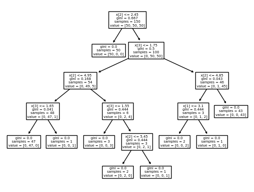
tree.plot_tree(clf)
[Text(0.5, 0.9166666666666666, 'x[2] <= 2.45\ngini = 0.667\nsamples = 150\nvalue = [50, 50, 50]'),
 Text(0.4230769230769231, 0.75, 'gini = 0.0\nsamples = 50\nvalue = [50, 0, 0]'),
 Text(0.5769230769230769, 0.75, 'x[3] <= 1.75\ngini = 0.5\nsamples = 100\nvalue = [0, 50, 50]'),
 Text(0.3076923076923077, 0.5833333333333334, 'x[2] <= 4.95\ngini = 0.168\nsamples = 54\nvalue = [0, 49, 5]'),
 Text(0.15384615384615385, 0.4166666666666667, 'x[3] <= 1.65\ngini = 0.041\nsamples = 48\nvalue = [0, 47, 1]'),
 Text(0.07692307692307693, 0.25, 'gini = 0.0\nsamples = 47\nvalue = [0, 47, 0]'),
 Text(0.23076923076923078, 0.25, 'gini = 0.0\nsamples = 1\nvalue = [0, 0, 1]'),
 Text(0.46153846153846156, 0.4166666666666667, 'x[3] <= 1.55\ngini = 0.444\nsamples = 6\nvalue = [0, 2, 4]'),
 Text(0.38461538461538464, 0.25, 'gini = 0.0\nsamples = 3\nvalue = [0, 0, 3]'),
 Text(0.5384615384615384, 0.25, 'x[2] <= 5.45\ngini = 0.444\nsamples = 3\nvalue = [0, 2, 1]'),
 Text(0.46153846153846156, 0.08333333333333333, 'gini = 0.0\nsamples = 2\nvalue = [0, 2, 0]'),
 Text(0.6153846153846154, 0.08333333333333333, 'gini = 0.0\nsamples = 1\nvalue = [0, 0, 1]'),
 Text(0.8461538461538461, 0.5833333333333334, 'x[2] <= 4.85\ngini = 0.043\nsamples = 46\nvalue = [0, 1, 45]'),
 Text(0.7692307692307693, 0.4166666666666667, 'x[1] <= 3.1\ngini = 0.444\nsamples = 3\nvalue = [0, 1, 2]'),
 Text(0.6923076923076923, 0.25, 'gini = 0.0\nsamples = 2\nvalue = [0, 0, 2]'),
 Text(0.8461538461538461, 0.25, 'gini = 0.0\nsamples = 1\nvalue = [0, 1, 0]'),
 Text(0.9230769230769231, 0.4166666666666667, 'gini = 0.0\nsamples = 43\nvalue = [0, 0, 43]')]
2.3.2 Otras opciones para graficar#
import plotly.express as px
df = px.data.iris()

fig = px.scatter_3d(
    df, x='sepal_length', y='sepal_width', z='petal_width',
    color='species',
    size = 'petal_length'
)

fig.show()
import graphviz
dot_data = tree.export_graphviz(clf, out_file=None)
graph = graphviz.Source(dot_data)
graph

2.3.4 Intentemos nosotros#
Probabilidades#
Si el objetivo es hacer clasificación sobre las clases $\(n_c \in \{0,1, \ldots, \mathrm{N}-1\}\)\(, para el nodo \)i\(, tenemos \)\( p_{i n_c}=\frac{1}{n_i} \sum_{y \in Q_i} I(y=n_c) \)$
Gini#
X, y = load_iris(return_X_y=True)
p_i_nc = lambda y, nc: 1/len(y)* np.sum(y == nc)
gini = lambda y, N: np.sum(np.sum(((p_i_nc(y, nc))*(1 - p_i_nc(y, nc)) for nc in N)))

2.3.4.a Primera iteración#
\(Q_i = \{1, \cdots, 150\}\) con \(\theta=(3, 0.8)\) el indice gini es:
gini(y, np.unique(y))
0.6666666666666667
2.3.4.b Segunda iteración#
dot_data = tree.export_graphviz(clf, out_file=None,
                      feature_names=iris.feature_names,
                     class_names=iris.target_names,
                     filled=True, rounded=True,
                     special_characters=True)
graph = graphviz.Source(dot_data)
graph

gini(y[X[:, 3] <= 0.8], np.unique(y[X[:, 3] <= 0.8]))
0.0
gini(y[X[:, 3] > 0.8], np.unique(y[X[:, 3] > 0.8]))
0.5
2.3.4.c Tercera iteración (izquierda)#

gini(y[(X[:, 3] > 0.8)&(X[:, 3] <= 1.75)], np.unique(y[(X[:, 3] > 0.8)&(X[:, 3] <= 1.75)]))
0.04079861111111115

gini(y[(X[:, 3] > 0.8)&(X[:, 3] <= 1.75)&(X[:, 2] <= 4.95)], np.unique(y[(X[:, 3] > 0.8)&(X[:, 3] <= 1.75)&(X[:, 2] <= 4.95)]))
2.5 Región de decisión#
2.5.1 Código#
Ejemplo tomado de Plot Iris DTC
import matplotlib.pyplot as plt
import numpy as np
from sklearn.datasets import load_iris
from sklearn.inspection import DecisionBoundaryDisplay
from sklearn.tree import DecisionTreeClassifier
# Parameters
n_classes = 3
plot_colors = "ryb"
plot_step = 0.02
for pairidx, pair in enumerate([[0, 1], [0, 2], [0, 3], [1, 2], [1, 3], [2, 3]]):
# We only take the two corresponding features
X = iris.data[:, pair]
y = iris.target
# Train
clf = DecisionTreeClassifier().fit(X, y)
# Plot the decision boundary
ax = plt.subplot(2, 3, pairidx + 1)
plt.tight_layout(h_pad=0.5, w_pad=0.5, pad=2.5)
DecisionBoundaryDisplay.from_estimator(
clf,
X,
cmap=plt.cm.RdYlBu,
response_method="predict",
ax=ax,
xlabel=iris.feature_names[pair[0]],
ylabel=iris.feature_names[pair[1]],
)
# Plot the training points
for i, color in zip(range(n_classes), plot_colors):
idx = np.where(y == i)
plt.scatter(
X[idx, 0],
X[idx, 1],
c=color,
label=iris.target_names[i],
cmap=plt.cm.RdYlBu,
edgecolor="black",
s=15,
)
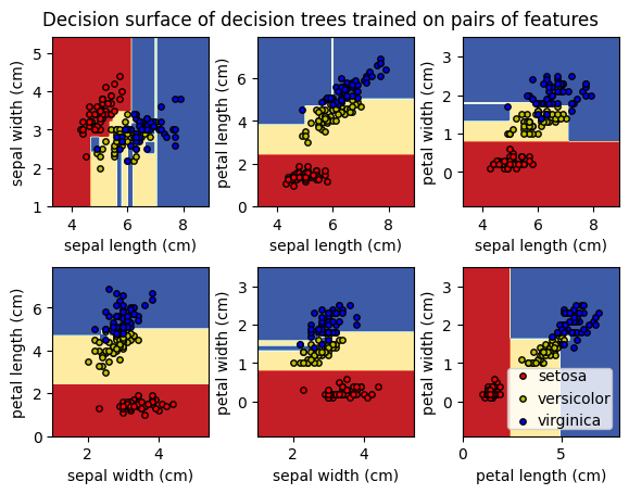
plt.suptitle("Decision surface of decision trees trained on pairs of features")
plt.legend(loc="lower right", borderpad=0, handletextpad=0)
_ = plt.axis("tight")