Introducción a métodos de regularización en Aprendizaje Automático

---------------------------------------------------------------------------
ModuleNotFoundError                       Traceback (most recent call last)
Cell In[1], line 1
----> 1 from tldraw import TldrawWidget
      2 t = TldrawWidget(width=1502, height = 700)

ModuleNotFoundError: No module named 'tldraw'

!pip install tldraw

Introducción a métodos de regularización en Aprendizaje Automático#

Versión b.1#

El notebook lo puedo modificar, esta versión es la b.1 a 05/06/2024 a las 17:13 Caracas.

Aprendizaje Automático [UCV]#

Autor: Fernando Crema García
Contacto: fernando.cremagarcia@kuleuven.be; fernando.cremagarcia@esat.kuleuven.be

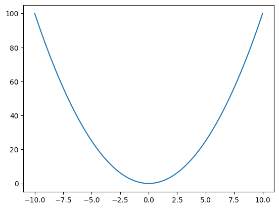
Plot de curva#

#@ plot_curve(f, _params=[], _range=(-5, 5), _points=100)

import matplotlib.pyplot as plt

def plot_curve(f, _params=[], _range=(-5, 5), _points=100):
  """
  Método para graficar una curva f(x) cuyos parámetros fijos son _params en el rango _range(min, max) usando subsampling de _points

  :param f: La función a graficar
  :param _params: Los parámetros fijos de la función
  :param _range: El rango de X (min, max)
  :param _points: Número de puntos donde vamos a subsamplear a f

  :returns: Nada
  """
  X = np.linspace(_range[0], _range[1], _points)
  plt.plot(X, np.array(list(map(lambda x: f(x, *_params), X))))

import numpy as np

f = lambda x, L, k, x0: L/(1.0 + np.exp(-1.0*k*(x-x0)))

f = lambda x: x**2

plot_curve(f, _range=(-10, 10))

../../_images/418b8d58e6433e2aa730fd0f110bc651f7afbe98dc9c98f9faf7f693666fe5ef.png

Resumen#

consideremos el problema de Regresión lineal : $$y = \mathbf{X} \beta_* + \epsilon \text{ with }$$

$\mathbf{X} \in \mathbb{R}^{n,m}$ a nuestra matriz de datos.
$\epsilon \in \mathbb{R}$ el ruido aleatorio definido como una variable aleatoria Normal con media $0$ y varianza $\sigma^2$, esto es, $\epsilon \sim \mathcal{N}(\mu=0,\,\sigma^{2})$
$y \in \mathbb{R}^n$ es nuestro vector a predecir que llamamos comunmente vector respuesta y del cual asumimos una relación lineal con $\mathbf{X}$.
$\beta_* \in \mathbb{R}^m$ es el modelo óptimo.

Supongamos que tenemos una muestra aleatoria de ($X, \mathbf{y}$) de tamaño $n$ para ambas $\mathbf{X}$ y $y$ entonces $X \in \mathbb{R}^{n \times m}$ y $\mathbf{y} \in \mathbb{R}^n$. El obketivo principal es conseguir $\beta_*$.

Definición: error $\hat{e}$#

Consideremos $\beta$ un estimador de $\beta_*$. Definimos el vector de error, $\hat{e}$, como: $$ \hat{e} = \mathbf{y} - X \beta $$

Definición: Un problema general de optimización $P(\lambda, s)$#

Definamos nuestro problema $P(\lambda, s)$ como:

\[P(\lambda,s)\;\;\underset{\beta,\mathbf{\hat{e}}}{min}\;\;f(\mathbf{\hat{e}}) + \lambda g(\beta)\;\;s.t.\]

\[\mathbf{y} - X \beta = \mathbf{\hat{e}}\]

\[h(\beta) \leq s\]

\[\mathbf{L} \leq A\beta \leq \mathbf{U}\]

\[\beta \in \mathbb{R}^m,\;\;y, \mathbf{\hat{e}} \in \mathbb{R}^n,\;\;X \in \mathbb{R}^{n \times m}\]

$f$ es la función de pérdida (loss function). Ejemplos típicos:

$f(\mathbf{\hat{e}}) = {\| \mathbf{\hat{e}} \|}_1$
$f(\mathbf{\hat{e}}) =\frac{1}{2} {\| \mathbf{\hat{e}} \|}^2_2$
Entre otros.

$h$ y $g$ las denominaremos funciones de complejidad del modelo $\beta$. Ejemplos típicos:
- $g(\mathbf{\beta}) = {\| \mathbf{\beta} \|}_1$ and $g(\mathbf{\beta}) = {\| \mathbf{\beta} \|}^2_2$
- $h(\mathbf{\beta}) = {\| \mathbf{\beta} \|}_1$ and $h(\beta) = {\| \beta \|}_0 = \vert \lbrace j: \beta_j \neq 0, j \in [n] \rbrace \vert$
- Entre otras.
Algunos elementos pueden desaparecer dependiendo de la formulación que necesitemos.

Motivo#

Normalmente intentamos minimizar el valor de una función de error, que denotaremos como $f$, para ser evaluada en $\hat{e}$ para encontrar buenos estimadores de $\beta_*$. Para lograr esto, agregamos una función de complejidad, que denotaremos como $g$ y $h$, que “controlará” el estimador $\hat{\beta}$ para ayudarnos a combatir el problema comúnmente conocido llamado sobreajuste. Hay varias formas de describir este problema.

Desde el punto de vista estadístico, la función de complejidad básicamente añade sesgo a nuestros estimadores con la ventaja de reducir su varianza. Esto significa que se encuentran mejores estimadores para que podamos generalizar mejor para datos desconocidos.
Desde un punto de vista no estadístico, la función de complejidad puede simplificar los estimadores (en el sentido de utilizar pocos regresores distintos de cero y/o con valores moderados) que nos permitan tener modelos fácilmente comprensibles.

Este proceso se conoce comúnmente como regularización

Regresión lineal (OLS)#

OLS ocurre con el siguiente setup:

$h = 0$, $\mathbf{L}=\mathbf{U}=g=A=\mathbf{0}$
$f(\mathbf{\hat{e}}) = {\frac{1}{2}\| \mathbf{\hat{e}} \|}^2_2$

Formulación de regresión lineal:#

En consecuencia, el problema a resolver es:

\[OLS\;\;\underset{\beta,\mathbf{\hat{e}}}{min}\;\;\frac{1}{2}\|\mathbf{\hat{e}}\|_2^2\;\;s.t.\]

\[\mathbf{y} - X \beta = \mathbf{\hat{e}}\]

\[\beta \in \mathbb{R}^m,\;\;y, \mathbf{\hat{e}} \in \mathbb{R}^n,\;\;X \in \mathbb{R}^{n \times m}\]

Solución analítica (Ecuaciones normales)#

\[ X^T X \beta = X^T y \Rightarrow \beta = (X^T X)^{-1}X^T y \]

LASSO#

Vamos a poner especial énfasis en el problema denominado LASSO [1].

Dado nuestro formato de formulación de problemas, Laso puede ser escrito como:

Forma lagrangeana:#

$h = 0$, $\mathbf{L}=\mathbf{U}=\mathbf{0}$
$A = \mathbf{0}$, $f(\mathbf{\hat{e}}) = {\frac{1}{2}\| \mathbf{\hat{e}} \|}^2_2$
$g(\mathbf{\beta}) = \lambda {\| \mathbf{\beta} \|}_1$.

Entonces, nuestro problema se convierte en:

\[Lasso(\lambda)\;\;\underset{\beta,\mathbf{\hat{e}}}{min}\;\; \frac{1}{2}\|\mathbf{\hat{e}}\|_2^2 + \lambda \|\beta\|_1\;\;s.t.\]

\[\mathbf{y} - X \beta = \mathbf{\hat{e}}\]

\[\beta \in \mathbb{R}^m,\;\;y, \mathbf{\hat{e}} \in \mathbb{R}^n,\;\;X \in \mathbb{R}^{n \times m}\]

Colocar biblliografía Hastie, Tibshirani Stanford

Forma con restricciones:#

$g = 0$, $\mathbf{L}=\mathbf{U}=\mathbf{0}$
$A = \mathbf{0}$, $f(\mathbf{\hat{e}}) = {\frac{1}{2}\| \mathbf{\hat{e}} \|}^2_2$
$h(\mathbf{\beta}) = {\| \mathbf{\beta} \|}_1$.

\[Lasso(s)\;\;\underset{\beta,\mathbf{\hat{e}}}{min}\;\;\frac{1}{2}\|\mathbf{\hat{e}}\|_2^2\;\;s.t.\]

\[\mathbf{y} - X \beta = \mathbf{\hat{e}}\]

\[{\| \mathbf{\beta} \|}_1 \leq s\]

\[\beta \in \mathbb{R}^m,\;\;y, \mathbf{\hat{e}} \in \mathbb{R}^n,\;\;X \in \mathbb{R}^{n \times m}\]

La regresión Lasso es un método de contracción (shrinkage). Lasso impone una penalidad $\ell_1$ en los parámetros $\beta$.

Lasso consigue el modelo óptimo para $\beta$ que minimiza la función

\[f(\beta) = \|y - X\beta \|_2^2 + \lambda \|\beta\|_1,\]

La penalización $\ell_1$ implica sparsidad “dispersidad” en los parámetros del modelo, y, como veremos, puede llevar muchos coeficientes al cero teórico. En este sentido, lasso es un método de selección de parámetros.

Closed form solution#

Si $X^{T} X=I,$ tenemos solución analítica: $\widehat{\beta}=S_{\lambda}\left(X^{T} y\right)$

Where $S_{\kappa}(a)=\left\{\begin{array}{ll}a-\kappa & a>\kappa \\ 0 & |a| \leq \kappa \\ a+\kappa & a<-\kappa\end{array}\right.$

Que es el famoso operador Soft-Thresholding.

Ridge regression#

También para este caso, tenemos dos posibles formulaciones. Para no extendernos más allá de una introducción, lo escribiremos en formulación lagrangeana.

Ridge: Formulación lagrangeana#

$h = 0$, $\mathbf{L}=\mathbf{U}=\mathbf{0}$
$A = \mathbf{0}$, $f(\mathbf{\hat{e}}) = {\frac{1}{2}\| \mathbf{\hat{e}} \|}^2_2$
$g(\mathbf{\beta}) = \lambda {\| \mathbf{\beta} \|}_2^2$.

Entonces, nuestro problema se convierte en:

\[Ridge(\lambda)\;\;\underset{\beta,\mathbf{\hat{e}}}{min}\;\; \frac{1}{2}\|\mathbf{\hat{e}}\|_2^2 + \lambda \|\beta\|_2^2\;\;s.t.\]

\[\mathbf{y} - X \beta = \mathbf{\hat{e}}\]

\[\beta \in \mathbb{R}^p,\;\;y, \mathbf{\hat{e}} \in \mathbb{R}^n,\;\;X \in \mathbb{R}^{n \times m}\]

Solución analítica#

\[\beta(\lambda)=\left(X^{\top} X+\lambda \mathbf{I}_{mm}\right)^{-1} X^{\top} y\]

Laboratorio#

!pip install cvxpy

Requirement already satisfied: cvxpy in /usr/local/lib/python3.10/dist-packages (1.3.4)
Requirement already satisfied: osqp>=0.4.1 in /usr/local/lib/python3.10/dist-packages (from cvxpy) (0.6.2.post8)
Requirement already satisfied: ecos>=2 in /usr/local/lib/python3.10/dist-packages (from cvxpy) (2.0.13)
Requirement already satisfied: scs>=1.1.6 in /usr/local/lib/python3.10/dist-packages (from cvxpy) (3.2.4.post2)
Requirement already satisfied: numpy>=1.15 in /usr/local/lib/python3.10/dist-packages (from cvxpy) (1.25.2)
Requirement already satisfied: scipy>=1.1.0 in /usr/local/lib/python3.10/dist-packages (from cvxpy) (1.11.4)
Requirement already satisfied: setuptools>65.5.1 in /usr/local/lib/python3.10/dist-packages (from cvxpy) (67.7.2)
Requirement already satisfied: qdldl in /usr/local/lib/python3.10/dist-packages (from osqp>=0.4.1->cvxpy) (0.1.7.post2)

from cvxpy import Variable, Problem, Minimize, Parameter
from cvxpy import sum_squares, norm2, matmul, norm1
import numpy as np
from sklearn.datasets import make_regression
import pandas as pd
import matplotlib.pyplot as plt

np.set_printoptions(suppress=True)

Generación de los datos#

Genere generate_data para crear una tupla X, y, w cuando el número de observaciones sea n, el número de características sea m y la proporción de coeficientes cero sea igual al density%. Por último, investigue la manera de settear el valor de la semilla seed.

def generate_data(n=20, m=5, sigma=0.3, density=0.2, seed=123456):
    "Generates data matrix X and observations Y."
    np.random.seed(seed)

    # Generación del modelo
    beta_star = sigma*np.random.randn(m)

    # Seleccionar los indices de sparcidad
    idxs = np.random.choice(range(m), int((1-density)*m), replace=False)

    # Setteando los valores exactamente a 0
    for idx in idxs:
        beta_star[idx] = 0

    # Creando la matriz del modelo N(0, sigma=1)
    X = np.random.randn(n, m)

    # Agregando ruido ~ N(0, sigma)
    Y = X.dot(beta_star) + np.random.normal(0, sigma, size=n)

    return X, Y.reshape(n, 1), beta_star.reshape(m, 1)

Tarea#

Utilice generate_data para crear la tupla X, y, w cuando el número de observaciones sea 30, el número de características sea 100 y la proporción de coeficientes cero sea igual al 90%.

_, _, _ = generate_data(n='', p='', density='')

---------------------------------------------------------------------------
TypeError                                 Traceback (most recent call last)
<ipython-input-9-1748bf4d4a80> in <cell line: 1>()
----> 1 _, _, _ = generate_data(n='', p='', density='')

TypeError: generate_data() got an unexpected keyword argument 'p'

Solution#

# 1224434
X, y, w = generate_data(n=30, m=100, sigma=3, density=0.1, seed=1232300)

TAREA: Cuántos problemas tienen más observaciones que entradas? Cómo se llaman este tipo de problemas?

array([[-0.63350035,  0.26295392,  0.76263251, ..., -0.64598602,
         0.6759692 ,  0.76589716],
       [-0.29670185, -1.24317874, -1.44805221, ..., -2.01568082,
         2.55138722, -1.38875027],
       [-1.38620007,  0.84080938, -1.24277066, ..., -0.71374822,
        -0.76373485, -0.19371327],
       ...,
       [ 0.96610246,  0.33565394, -0.00787418, ...,  0.75958059,
        -0.07645028,  1.21636902],
       [ 0.16995524, -0.94485736,  3.01347295, ..., -1.15095968,
        -0.57994119, -0.97079591],
       [ 1.19477043, -1.08379873, -0.5747683 , ...,  2.12015979,
        -0.37308524, -0.09980036]])

X.shape

(30, 100)

y.shape

(30, 1)

array([[ 0.        ],
       [ 0.        ],
       [-2.12078223],
       [ 0.        ],
       [ 4.8878188 ],
       [ 0.        ],
       [ 0.        ],
       [ 0.        ],
       [ 0.        ],
       [ 0.        ],
       [ 0.        ],
       [ 0.        ],
       [ 0.        ],
       [ 0.        ],
       [ 0.        ],
       [ 0.        ],
       [ 0.        ],
       [ 0.        ],
       [ 0.        ],
       [ 0.        ],
       [ 0.        ],
       [-4.11227443],
       [ 0.        ],
       [ 0.        ],
       [ 0.        ],
       [ 0.        ],
       [ 0.        ],
       [ 0.        ],
       [ 0.        ],
       [ 0.        ],
       [ 0.        ],
       [ 0.8450862 ],
       [ 0.        ],
       [ 0.        ],
       [ 0.        ],
       [ 0.        ],
       [ 0.        ],
       [ 0.        ],
       [ 0.        ],
       [ 0.        ],
       [ 0.        ],
       [ 0.        ],
       [ 0.        ],
       [ 0.        ],
       [ 0.        ],
       [ 0.        ],
       [ 0.        ],
       [ 0.        ],
       [ 0.        ],
       [ 0.        ],
       [ 0.        ],
       [ 0.        ],
       [ 0.        ],
       [ 0.        ],
       [ 0.        ],
       [ 0.        ],
       [ 0.        ],
       [ 0.        ],
       [ 0.        ],
       [ 0.        ],
       [ 0.        ],
       [ 0.        ],
       [ 0.        ],
       [ 0.        ],
       [ 0.        ],
       [ 0.        ],
       [ 0.        ],
       [ 0.        ],
       [ 0.        ],
       [ 0.        ],
       [ 0.        ],
       [ 0.        ],
       [ 0.        ],
       [ 0.        ],
       [ 0.        ],
       [ 0.        ],
       [ 0.        ],
       [ 0.        ],
       [ 0.        ],
       [ 0.        ],
       [ 0.        ],
       [ 0.        ],
       [ 3.82534953],
       [ 0.56192792],
       [ 0.        ],
       [ 0.        ],
       [ 2.80061345],
       [ 0.        ],
       [ 0.        ],
       [ 0.        ],
       [ 0.        ],
       [ 0.        ],
       [ 0.        ],
       [ 0.01574646],
       [ 0.        ],
       [ 0.        ],
       [-3.63232242],
       [ 0.        ],
       [ 0.        ],
       [-3.06562084]])

n, m = 50, 100

X, y, w = make_regression(n_samples=n, n_features=m, n_informative=10, noise=1, random_state=1232300, coef=True)

y = y.reshape(n, 1)

Generación del modelo#

Usaremos el famoso paquete CVXPY de la Universidad de Stanford porque nos permite expresar su problema de una manera natural que sigue las matemáticas, en lugar de la forma estándar restrictiva requerida por paquetes denominados solvers (Gurobi, CPLEX, etcétera).

Para obtener más información, visite la página web principal CVX donde explicaron más sobre la programación convexa disciplinada.

Ordinary Least Squares#

(n, m), solver = X.shape, None

X_ols = Parameter(shape=X.shape, name="X")
y_ols = Parameter(shape=y.shape, name="y")
w_ols = Variable(shape=(m, 1), name="w_ols")

X_ols.value, y_ols.value = X, y

ols = Problem(
    Minimize
    (
        sum_squares(y_ols - X_ols@w_ols)
    )
)

if solver is not None:
    ols.solve(solver=solver)
else:
    ols.solve()

coef_ols = w_ols.value

coef_ols

Lasso: Formulación con restricciones#

(n, m), solver, s = X.shape, None, 13.30309405261565

X_lasso = Parameter(shape=X.shape, name="X")
y_lasso = Parameter(shape=y.shape, name="y")
s_lasso = Parameter(nonneg=True, name="s")
w_lasso = Variable(shape=(m, 1), name="w_lasso")

X_lasso.value, y_lasso.value, s_lasso.value = X, y, s

Lasso = Problem(
    Minimize(
        norm2(y_lasso - X_lasso@w_lasso)**2
    ),
    [norm1(w_lasso) <= s_lasso]
)

if solver is not None:
    Lasso.solve(solver=solver)
else:
    Lasso.solve()

coef_lasso = w_lasso.value

for lasso, opt in zip(coef_lasso, w):
  print("lasso: {} opt: {}".format(lasso, opt))

lasso: [-0.] opt: [0.]
lasso: [0.11283356] opt: [0.]
lasso: [-1.19240377] opt: [-2.12078223]
lasso: [-0.00000002] opt: [0.]
lasso: [3.19427519] opt: [4.8878188]
lasso: [-0.] opt: [0.]
lasso: [0.00000001] opt: [0.]
lasso: [-0.] opt: [0.]
lasso: [-0.] opt: [0.]
lasso: [-0.] opt: [0.]
lasso: [0.00000001] opt: [0.]
lasso: [0.] opt: [0.]
lasso: [0.] opt: [0.]
lasso: [0.] opt: [0.]
lasso: [0.00000001] opt: [0.]
lasso: [0.] opt: [0.]
lasso: [0.] opt: [0.]
lasso: [0.] opt: [0.]
lasso: [-0.] opt: [0.]
lasso: [-0.] opt: [0.]
lasso: [-0.] opt: [0.]
lasso: [-3.59080159] opt: [-4.11227443]
lasso: [-0.] opt: [0.]
lasso: [0.00000001] opt: [0.]
lasso: [-0.] opt: [0.]
lasso: [-0.] opt: [0.]
lasso: [0.] opt: [0.]
lasso: [-0.00000001] opt: [0.]
lasso: [-0.] opt: [0.]
lasso: [0.00000001] opt: [0.]
lasso: [0.] opt: [0.]
lasso: [0.00000001] opt: [0.8450862]
lasso: [-0.] opt: [0.]
lasso: [-0.] opt: [0.]
lasso: [-0.] opt: [0.]
lasso: [0.00000001] opt: [0.]
lasso: [-0.] opt: [0.]
lasso: [-0.00000002] opt: [0.]
lasso: [-0.] opt: [0.]
lasso: [-0.] opt: [0.]
lasso: [-0.] opt: [0.]
lasso: [0.] opt: [0.]
lasso: [0.] opt: [0.]
lasso: [-0.] opt: [0.]
lasso: [0.] opt: [0.]
lasso: [-0.] opt: [0.]
lasso: [-0.00000003] opt: [0.]
lasso: [-0.] opt: [0.]
lasso: [-0.] opt: [0.]
lasso: [-0.] opt: [0.]
lasso: [0.] opt: [0.]
lasso: [0.] opt: [0.]
lasso: [-0.] opt: [0.]
lasso: [0.00000001] opt: [0.]
lasso: [0.] opt: [0.]
lasso: [-0.] opt: [0.]
lasso: [-0.00000001] opt: [0.]
lasso: [0.] opt: [0.]
lasso: [0.00000001] opt: [0.]
lasso: [0.00000002] opt: [0.]
lasso: [0.] opt: [0.]
lasso: [0.] opt: [0.]
lasso: [-0.] opt: [0.]
lasso: [0.] opt: [0.]
lasso: [-0.00000004] opt: [0.]
lasso: [-0.00000001] opt: [0.]
lasso: [0.] opt: [0.]
lasso: [0.] opt: [0.]
lasso: [-0.] opt: [0.]
lasso: [-0.] opt: [0.]
lasso: [-0.] opt: [0.]
lasso: [-0.] opt: [0.]
lasso: [-0.] opt: [0.]
lasso: [-0.] opt: [0.]
lasso: [-0.] opt: [0.]
lasso: [-0.16919671] opt: [0.]
lasso: [-0.] opt: [0.]
lasso: [-0.00000001] opt: [0.]
lasso: [0.] opt: [0.]
lasso: [0.00000001] opt: [0.]
lasso: [-0.00000001] opt: [0.]
lasso: [-0.] opt: [0.]
lasso: [3.37050329] opt: [3.82534953]
lasso: [0.00000001] opt: [0.56192792]
lasso: [0.] opt: [0.]
lasso: [-0.] opt: [0.]
lasso: [0.00000001] opt: [2.80061345]
lasso: [0.00000001] opt: [0.]
lasso: [0.00000001] opt: [0.]
lasso: [-0.22078036] opt: [0.]
lasso: [-0.] opt: [0.]
lasso: [0.] opt: [0.]
lasso: [-0.00000001] opt: [0.]
lasso: [0.] opt: [0.01574646]
lasso: [-0.00000001] opt: [0.]
lasso: [0.] opt: [0.]
lasso: [-1.75139798] opt: [-3.63232242]
lasso: [-0.] opt: [0.]
lasso: [-0.] opt: [0.]
lasso: [-1.70090119] opt: [-3.06562084]

Lasso: Formulación lagrangeana#

(n, m), solver, Lambda = X.shape, None, 12.329764280592936

X_lasso_lag = Parameter(shape=X.shape, name="X")
y_lasso_lag = Parameter(shape=y.shape, name="y")
L_lasso_lag = Parameter(nonneg=True, name="Lambda")
w_lasso_lag = Variable(shape=(m, 1), name="w_ols")

X_lasso_lag.value, y_lasso_lag.value, L_lasso_lag.value = X, y, Lambda

Lasso_lag = Problem(
    Minimize(
        sum_squares(y_lasso_lag - X_lasso_lag@w_lasso_lag) + L_lasso_lag*norm1(w_lasso_lag)
    )
)

if solver is not None:
    Lasso_lag.solve(solver=solver)
else:
    Lasso_lag.solve()

coef_lasso_lag = w_lasso_lag.value

Ver resultados básicos#

pd.set_option('display.float_format', str)

from re import M
df = pd.DataFrame.from_dict(
    {
        "w": w.reshape(m),
        "OLS": coef_ols.reshape(m),
        "Constrained": coef_lasso.reshape(m),
        "Lagrangian": coef_lasso_lag.reshape(m)
    }
)

df[np.abs(df.w)>0]

	w	OLS	Constrained	Lagrangian
2	-2.120782	-1.298915	-1.192404e+00	-2.352770e+00
4	4.887819	2.214128	3.194275e+00	3.689219e+00
21	-4.112274	-1.939734	-3.590802e+00	-3.160052e+00
31	0.845086	-0.381689	5.391194e-09	1.290389e-20
82	3.825350	1.398275	3.370503e+00	3.753718e+00
83	0.561928	1.037364	1.227250e-08	8.032137e-01
86	2.800613	0.786181	1.279780e-08	9.699106e-01
93	0.015746	0.200665	4.371577e-09	7.083847e-03
96	-3.632322	-1.741400	-1.751398e+00	-2.445004e+00
99	-3.065621	-2.183951	-1.700901e+00	-3.056797e+00

Calculando el camino de regularización y los valores cuadráticos medios#

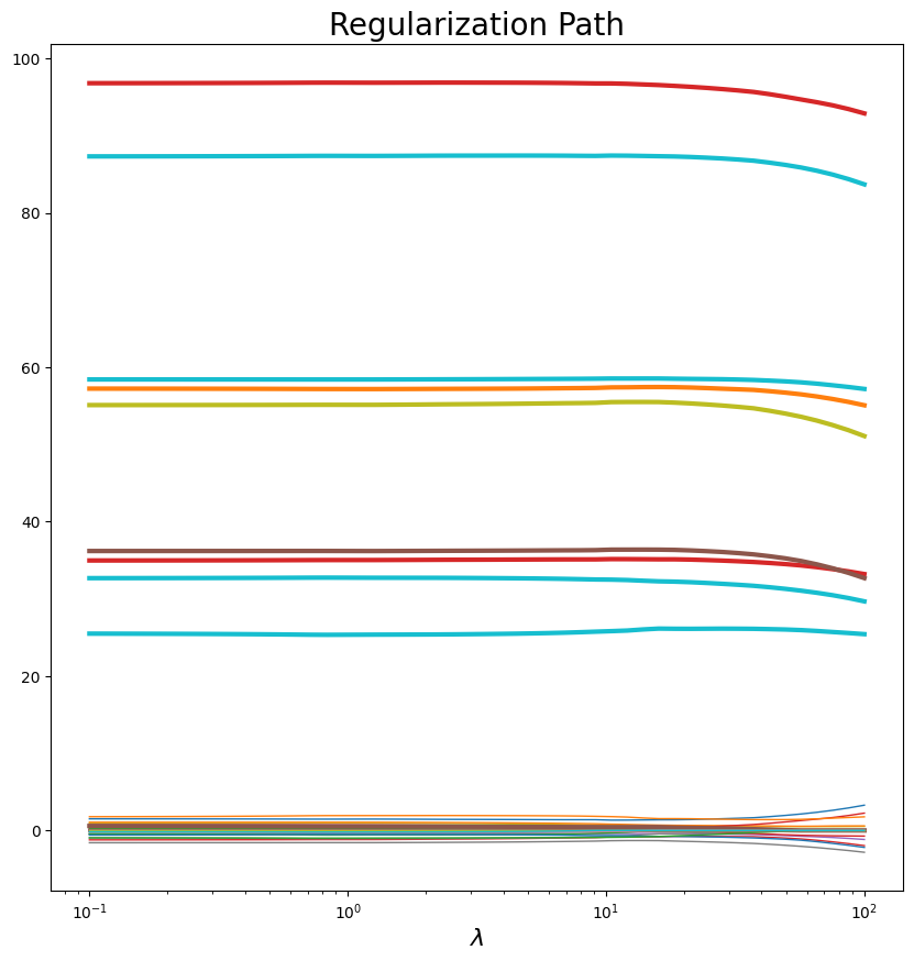
Ahora, usemos solo la formulación lagrangiana de Lasso, terminemos el script a continuación para que podamos trazar el camino de regularización dadas las lambdas proporcionadas.

regularization path

Métodos#

Mean Squared Error (MSE)#

def mse(X, y, beta):
    """This function computes the mean squared value given a Model Matrix X, a response vector y and a model beta.
    Args:
        X (numpy.ndarray): [description]
        y (numpy.array): [description]
        beta (numpy.array): [description]
    Returns:
        float: The mean squared error
    """
    return (1.0 / X.shape[0]) * loss_fn(X, y, beta).value

Loss function#

def loss_fn(X, y, beta):
    """Calculates the value of the loss function
    Args:
        X (numpy.ndarray): [description]
        y (numpy.array): [description]
        beta (numpy.array): [description]
    Returns:
        float: The loss function evaluated at beta
    """
    return norm2(X @ beta - y)**2

Sección de gráficos#

Esta sección provee código para visualización de métodos comunes.

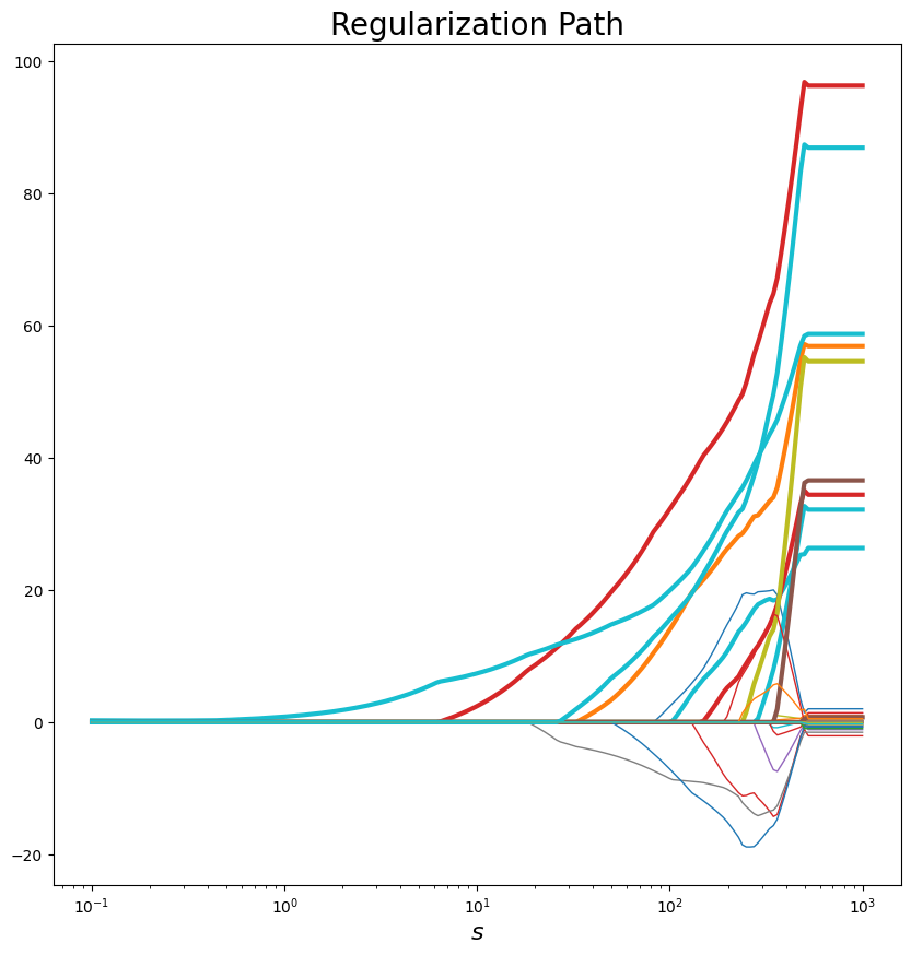
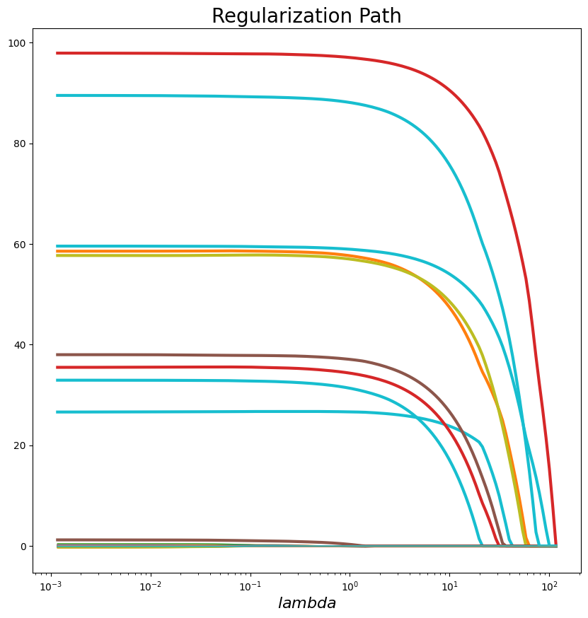
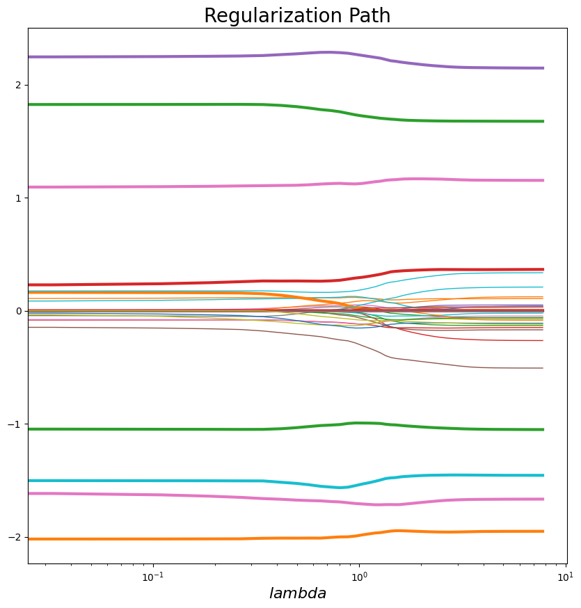
Regularization path#

def plot_regularization_path(lambd_values, beta_values, true_features, legend="\lambda", title="Regularization Path"):
    """Method to plot the regularization path given lambda values and beta values
    Args:
        lambd_values (numpy.ndarray): An array of lambda values
        beta_values (numpy.ndarray): A matrix of size (n, lambdas) with n the number of lambdas.
        legend (str): The x-axis label of interest (Defaults to lambda).
        title (str): The plot title name (Defaults to Regularization Path)
    """
    num_coeffs = len(beta_values[0])
    plt.figure(figsize=(10,10))
    for i in range(num_coeffs):
        plt.plot(lambd_values, [wi[i] for wi in beta_values], linewidth=3 if i in true_features else 1)
    plt.xlabel(r"${}$".format(legend), fontsize=16)
    plt.xscale("log")
    plt.title("{}".format(title), fontsize=20)
    plt.show()

Mean Squared Error (MSE)#

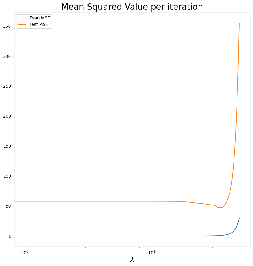
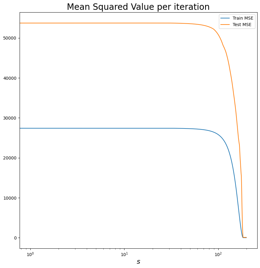
def plot_mse(train_mse, test_mse, legend="\lambda", title="Mean Squared Value per iteration"):
    """Ploting the MSE per iteration
    Args:
        train__mse (numpy.ndarray): The array with the mse values related to the training set
        test__mse (numpy.ndarray): The array with the mse values related to the test set
        legend (str): The x-axis label of interest (Defaults to lambda).
        title (str): The plot title name (Mean Squared Value per iteration)
    """
    plt.figure(figsize=(10,10))
    plt.plot(range(len(train_mse)), train_mse)
    plt.plot(range(len(test_mse)), test_mse)
    plt.xlabel(r"${}$".format(legend), fontsize=16)
    plt.xscale("log")
    plt.title("{}".format(title), fontsize=20)
    plt.legend(['Train MSE', 'Test MSE'])
    plt.show()

Tarea#

Primero, dividamos los datos usando la forma más básica: 70% para el conjunto de entrenamiento y 30% para el conjunto de prueba. Posteriormente calcularemos el camino de regularización para ambas formulaciones.

Su tarea es rehacer la formulación para la forma restringida dada la solución de la forma lagrangiana.

Ya calculamos los conjuntos de datos X e y tanto para el entrenamiento como para las pruebas.

¿Por qué los trazados de las rutas de regularización son diferentes?
¿Por qué la MSE cambia dependiendo de los esquemas de train y test?
¿Qué lambda deberíamos elegir? ¿Cómo ayudarnos a hacer esto?
Preste atención a las unidades de las lambdas, s. ¿Que estamos haciendo? ¿Por qué?

(n_total, p_total), solver, Lambda, split = X.shape, None, 2.0, 0.3

k = int(n_total * (1 - split))

X_train, X_test, y_train, y_test  = X[:k, :], X[k:, :], y[:k], y[k:]

X_train

array([[-0.63350035,  0.26295392,  0.76263251, ..., -0.64598602,
         0.6759692 ,  0.76589716],
       [-0.29670185, -1.24317874, -1.44805221, ..., -2.01568082,
         2.55138722, -1.38875027],
       [-1.38620007,  0.84080938, -1.24277066, ..., -0.71374822,
        -0.76373485, -0.19371327],
       ...,
       [-0.52409478,  1.85497963,  0.45653019, ..., -0.2768307 ,
         1.34434149, -0.24048937],
       [-0.43690786,  0.02388454, -1.13004838, ..., -1.01631585,
        -2.10078725, -0.53722419],
       [ 0.19356863,  0.34666492,  0.84401141, ..., -0.10603981,
        -0.28806073,  1.0953223 ]])

Lasso con lagrangian formulation#

X_lasso_lag = Parameter(shape=X_train.shape, name="X")
y_lasso_lag = Parameter(shape=y_train.shape, name="y")
L_lasso_lag = Parameter(nonneg=True, name="Lambda")
w_lasso_lag = Variable(shape=(p_total, 1), name="w_ols")

X_lasso_lag.value, y_lasso_lag.value = X_train, y_train

Lasso_lag = Problem(
    Minimize(
        norm2(y_lasso_lag - X_lasso_lag@w_lasso_lag)**2 + L_lasso_lag*norm1(w_lasso_lag)
    )
)

lambda_values = np.logspace(-1, 2, 50)
w_values, train_mse_values_lag, test_mse_values_lag = [], [], []

for l in lambda_values:
    L_lasso_lag.value = l
    Lasso_lag.solve()
    w_values.append(w_lasso_lag.value)
    train_mse_values_lag.append(mse(X=X_train, y=y_train, beta=w_lasso_lag.value))
    test_mse_values_lag.append(mse(X=X_test, y=y_test, beta=w_lasso_lag.value))

np.log10(np.flip(lambda_values))

array([ 2.        ,  1.93877551,  1.87755102,  1.81632653,  1.75510204,
        1.69387755,  1.63265306,  1.57142857,  1.51020408,  1.44897959,
        1.3877551 ,  1.32653061,  1.26530612,  1.20408163,  1.14285714,
        1.08163265,  1.02040816,  0.95918367,  0.89795918,  0.83673469,
        0.7755102 ,  0.71428571,  0.65306122,  0.59183673,  0.53061224,
        0.46938776,  0.40816327,  0.34693878,  0.28571429,  0.2244898 ,
        0.16326531,  0.10204082,  0.04081633, -0.02040816, -0.08163265,
       -0.14285714, -0.20408163, -0.26530612, -0.32653061, -0.3877551 ,
       -0.44897959, -0.51020408, -0.57142857, -0.63265306, -0.69387755,
       -0.75510204, -0.81632653, -0.87755102, -0.93877551, -1.        ])

plot_regularization_path(lambda_values, w_values, df[np.abs(df.w)>0].index.values)

../../_images/537ac7d86796a28ade59b5acfe177e600af4dad3f7e4867f7760f1cb7a7ff627.png

lambda_values

array([  0.1       ,   0.11513954,   0.13257114,   0.1526418 ,
         0.17575106,   0.20235896,   0.23299518,   0.26826958,
         0.30888436,   0.35564803,   0.40949151,   0.47148664,
         0.54286754,   0.62505519,   0.71968567,   0.82864277,
         0.95409548,   1.09854114,   1.26485522,   1.45634848,
         1.67683294,   1.93069773,   2.22299648,   2.55954792,
         2.9470517 ,   3.39322177,   3.90693994,   4.49843267,
         5.17947468,   5.96362332,   6.86648845,   7.90604321,
         9.10298178,  10.48113134,  12.06792641,  13.89495494,
        15.9985872 ,  18.42069969,  21.20950888,  24.42053095,
        28.11768698,  32.37457543,  37.2759372 ,  42.9193426 ,
        49.41713361,  56.89866029,  65.51285569,  75.43120063,
        86.85113738, 100.        ])

plot_mse(train_mse_values_lag, test_mse_values_lag)

../../_images/f8c12126890462340946b0093a16ab3dbe9838a3a4ccf2e75dac7567097dbb02.png

Solution (Lasso with constrained formulation)#

X_lasso = Parameter(shape=X_train.shape, name="X")
y_lasso = Parameter(shape=y_train.shape, name="y")
s_lasso = Parameter(nonneg=True, name="s")
w_lasso = Variable(shape=(p_total, 1), name="w_lasso")

X_lasso.value, y_lasso.value = X_train, y_train

Lasso = Problem(
    Minimize(
        sum_squares(y_lasso - X_lasso@w_lasso)
    ),
    [norm1(w_lasso) <= s_lasso]
)

s_values = np.logspace(-1, 3, 200)
w_values, train_mse_values, test_mse_values = [], [], []

for s in s_values:
    s_lasso.value = s
    Lasso.solve()
    w_values.append(w_lasso.value)
    train_mse_values.append(mse(X=X_train, y=y_train, beta=w_lasso.value))
    test_mse_values.append(mse(X=X_test, y=y_test, beta=w_lasso.value))

plot_regularization_path(s_values, w_values, df[np.abs(df.w)>0].index.values, legend="s")

../../_images/33435fe4b8ab4969b643766e4a59cf68cdeab837b201e8b109ee93281c7d4f4a.png

plot_mse(train_mse_values, test_mse_values, legend="s")

../../_images/a2e9ccf81fc9ea7ff859c8e30bb388e3e339ed2b7bc101900ef9116ece7c2b46.png

Selección de modelo: Eligiendo las mejores lambda y s#

Para nuestro esquema de selección de modelo, debemos elegir la lambda, s que minimice el error cuadrático medio en el conjunto de prueba.

s_values[np.argmin(test_mse_values)]

499.450511585514

lambda_values[np.argmin(test_mse_values_lag)]

13.894954943731374

Resumen de resultados#

df[np.abs(df.w)>0].index.values

array([19, 21, 23, 29, 33, 48, 59, 65, 75, 79])

df.head(20)

	w	OLS	Constrained	Lagrangian
0	0.0	3.9294838821971894	7.95995528711988e-06	0.07867077883679029
1	0.0	5.889413081539131	3.0537798060713576e-06	0.0624234323648013
2	0.0	-26.045169243014566	-1.282998482939311e-05	1.2555561326594936e-20
3	0.0	-10.673939019622233	-4.5968229882094525e-05	1.7551389601218054e-20
4	0.0	-2.8673253654092807	-3.861927665245822e-06	3.080455159479548e-20
5	0.0	-20.54033881927282	-4.054337357283422e-06	-1.5286153248773428e-20
6	0.0	10.524865217399817	3.874090036884144e-06	3.431325693888233e-20
7	0.0	18.439708715668175	4.191689310136686e-06	-2.5013015165473396e-20
8	0.0	-5.159176292532276	-3.0439777958382878e-06	1.3264509758520135e-20
9	0.0	-0.8635817193402358	4.687750763150862e-06	1.943226118192214e-20
10	0.0	16.34016963909085	1.2936342879974396e-05	6.211325455869969e-21
11	0.0	-2.9502578993941095	4.015629972049802e-06	-3.7849452363988635e-21
12	0.0	-4.866954673669433	-3.676366135359239e-06	-6.66730256582179e-21
13	0.0	6.950858041770783	1.2422589165861853e-05	1.7907932222695616e-20
14	0.0	-11.583829883992935	-3.45786468513482e-06	2.9766593203452626e-20
15	0.0	12.556810519279312	7.453404670799487e-06	-2.160140464454571e-20
16	0.0	0.4062769118807657	-3.077741548518156e-06	-2.903613006387567e-21
17	0.0	-16.69890339089355	-2.0966113707555978e-06	1.2266652978297838e-20
18	0.0	5.4930472743317145	1.1572912528642797e-05	-3.814055666211338e-20
19	26.79571437692997	10.613187251165535	1.6423880340491963e-05	26.70365724383208

Frameworks en producción (Real World)#

Aunque cvx es extremadamente útil, cuando buscamos modelos con regularización (usando Python) tendemos a usar otros frameworks.

Aquí, además del framework del curso Scikit-Learnexisten otros paquetes como [GLMnet] de Stanford (https://web.stanford.edu/~hastie/glmnet_python/), [Tensorflow] de Google (https://www.tensorflow.org/) y [PyTorch] de Facebook (https ://pytorch.org/).

Usando Scikit-Learn#

Existen muchos métodos que podemos utilizar pero LassoCV es el más usado en producción porque estamos haciendo al mismo tiempo selección de modelos y consiguiendo el modelo óptimo en base a ciertos parámetros.

Import library#

from sklearn.linear_model import LassoCV

Attributes#

alpha (float): The amount of penalization chosen by cross validation
coef (ndarray of shape (n_features,) or (ntargets, n_features)) parameter vector (w in the cost function formula)
intercept (float or ndarray of shape (ntargets,): independent term in decision function.
mse_path ndarray of shape (n_alphas, n_folds): mean square error for the test set on each fold, varying alpha
alphas (ndarray of shape (n_alphas,): The grid of alphas used for fitting
dual_gap (float or ndarray of shape (ntargets,)) The dual gap at the end of the optimization for the optimal alpha (alpha_).
n_iter (int number of iterations): run by the coordinate descent solver to reach the specified tolerance for the optimal alpha.

Methods#

fit(X, y): Fit linear model with coordinate descent
get_params([deep]): Get parameters for this estimator.
path(X, y, *[, eps, n_alphas, alphas, …]): Compute Lasso path with coordinate descent
predict(X): Predict using the linear model.
score(X, y[, sample_weight]): Return the coefficient of determination R^2 of the prediction.
set_params(**params): Set the parameters of this estimator.

Model selection via k-fold cross validation#

model = LassoCV(cv=7, random_state=1232300).fit(X, y.reshape(n))

from sklearn.linear_model import enet_path, lasso_path

eps = 5e-3  # the smaller it is the longer is the path

print("Computing regularization path using the lasso...")
alphas_lasso, coefs_lasso, _ = lasso_path(X, y, eps=eps)

Computing regularization path using the lasso...

coefs_lasso.shape

(1, 100, 100)

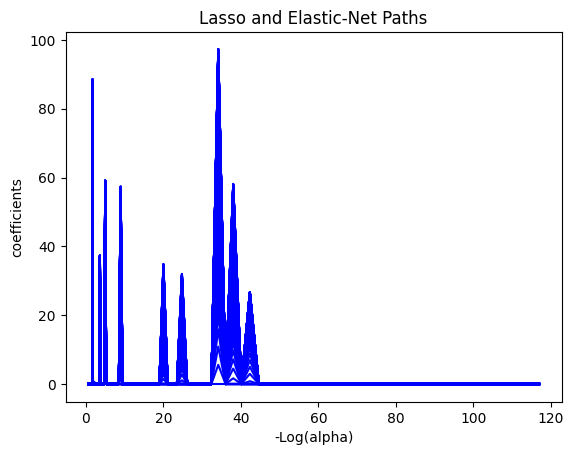
from itertools import cycle
plt.figure(1)
colors = cycle(["b", "r", "g", "c", "k"])
neg_log_alphas_lasso = alphas_lasso
for coef_l, c in zip(coefs_lasso, colors):
  print(c, coef_l)
  l1 = plt.plot(neg_log_alphas_lasso, coef_l, c=c)
plt.xlabel("-Log(alpha)")
plt.ylabel("coefficients")
plt.title("Lasso and Elastic-Net Paths")
plt.axis("tight")

b [[0. 0. 0. ... 0. 0. 0.]
 [0. 0. 0. ... 0. 0. 0.]
 [0. 0. 0. ... 0. 0. 0.]
 ...
 [0. 0. 0. ... 0. 0. 0.]
 [0. 0. 0. ... 0. 0. 0.]
 [0. 0. 0. ... 0. 0. 0.]]

(-5.235093010806908,
 122.80533828144249,
 -5.148408483834903,
 102.27550132897926)

../../_images/5a42c20ba1cb59929df2f02533fd2ccfe6d6bad0900a32110d3928e81331ea2e.png

 coefs_lasso.shape

(1, 100, 100)

New Section#

alphas_lasso

array([116.98531868, 110.88904295, 105.11045305,  99.6329939 ,
        94.44097315,  89.51951618,  84.85452351,  80.43263042,
        76.24116864,  72.26813005,  68.50213229,  64.93238618,
        61.54866475,  58.34127398,  55.30102503,  52.41920789,
        49.68756645,  47.09827483,  44.64391497,  42.31745539,
        40.11223102,  38.02192411,  36.04054614,  34.16242067,
        32.38216706,  30.69468506,  29.09514022,  27.57894999,
        26.14177064,  24.77948482,  23.48818969,  22.26418584,
        21.10396661,  20.00420811,  18.96175962,  17.97363465,
        17.03700231,  16.14917925,  15.30762194,  14.50991942,
        13.75378633,  13.03705645,  12.35767641,  11.71369985,
        11.10328185,  10.52467363,   9.97621752,   9.45634226,
         8.96355846,   8.49645435,   8.05369171,   7.63400208,
         7.23618308,   6.85909502,   6.50165757,   6.1628467 ,
         5.84169176,   5.53727268,   5.24871731,   4.97519899,
         4.71593411,   4.4701799 ,   4.2372323 ,   4.01642394,
         3.80712223,   3.60872753,   3.42067147,   3.24241529,
         3.07344829,   2.91328641,   2.76147081,   2.61756653,
         2.48116132,   2.35186438,   2.22930529,   2.11313294,
         2.0030145 ,   1.89863449,   1.79969387,   1.7059092 ,
         1.61701178,   1.53274694,   1.45287326,   1.37716191,
         1.30539599,   1.2373699 ,   1.17288875,   1.11176781,
         1.05383196,   0.99891524,   0.94686031,   0.89751804,
         0.85074706,   0.80641339,   0.76439001,   0.72455653,
         0.68679883,   0.65100874,   0.61708373,   0.58492659])

best = model.coef_

Agregando columna al data frame de soluciones#

df = pd.DataFrame.from_dict(
    {
        "w": w.reshape(m),
        "OLS": coef_ols.reshape(m),
        "Constrained": coef_lasso.reshape(m),
        "Lagrangian": coef_lasso_lag.reshape(m),
        "LassoCV": best
    }
)

df[np.abs(df.w)>0]

	w	OLS	Constrained	Lagrangian	LassoCV
19	26.79571437692997	10.613187251165535	1.6423880340491963e-05	26.70365724383208	26.787188100892624
21	58.67947690864924	44.92352862709617	4.1489004152348326	58.57441987443998	58.49817705665139
23	97.83431853646809	61.49454785217981	55.129045875649396	97.76220328661873	97.784215064098
29	33.02340993896776	22.61834243976383	3.2430295772288494e-06	32.74304109457136	32.68080495115607
33	35.8839221732842	15.842341333054673	1.5255369935423097e-05	35.51292548126903	35.471625701064646
48	58.01220830471275	34.10976978845665	1.4464192149246933	57.80391161426959	57.80702788245752
59	59.56291123952296	32.27312300387868	23.41657727934535	59.478421150185135	59.47487127655933
65	38.15924099685708	26.10672638162152	1.8636527432986245e-05	37.833536027361674	37.79070788789274
75	0.9260389671008395	-1.6937118794019477	2.1917397086653213e-06	1.0184959689381567	0.9316665243873982
79	89.48445234796701	59.57671177507784	23.16049748562707	89.21607703653586	89.24750532684156

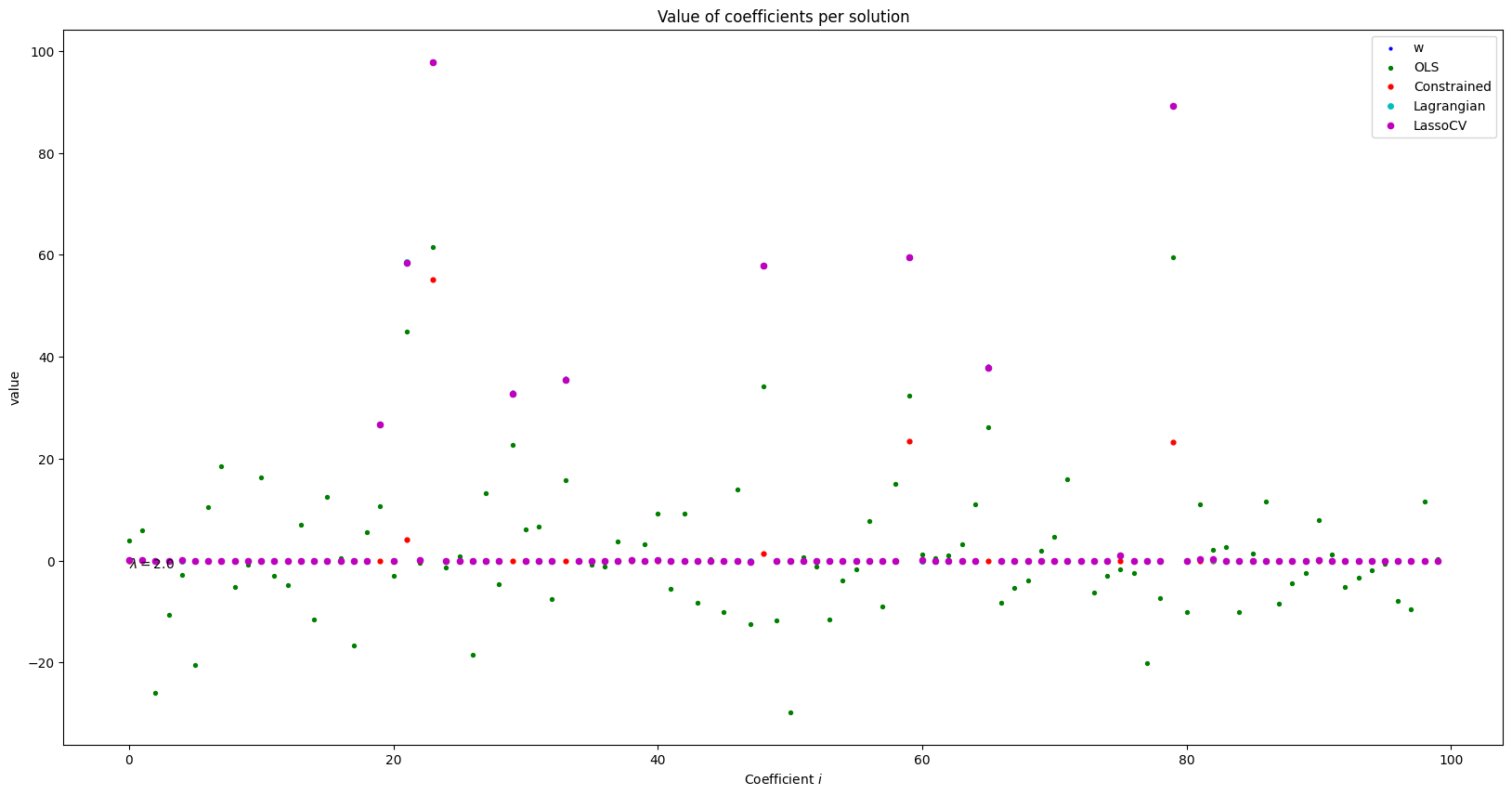
Comparando los valores de los coeficientes#

def plot_coefficients(plot_info, w=20, h=10):
    """[summary]
    Args:
        plot_info ([type]): [description]
    """
    plt.figure(figsize=(w, h))
    for label, value in plot_info.items():
        plt.scatter(
            range(len(value["w"])),
            value["w"],
            label=label,
            c=value["color"],
            s=value["size"]
        )
    plt.text(0.0, -1.5, r"$\lambda={:3}$".format(Lambda))
    plt.title("Value of coefficients per solution")
    plt.ylabel("value")
    plt.xlabel(r"Coefficient $i$")
    plt.legend()
    plt.show()

cmaps = ['b', 'g', 'r', 'c', 'm', 'y', 'k'] # https://matplotlib.org/3.1.0/tutorials/colors/colormaps.html
to_plot = {
    k: {
        "color": cmaps[i%len(cmaps)], "size": 4 + i*4, "w": w.values
    } for i, (k, w) in enumerate(df.items())
}

plot_coefficients(plot_info=to_plot)

../../_images/928776a56fa8aef1f79073e44ef92e8274fc545aa7d2d16e463ba8f76de2100d.png

Regularization path per each fold#

We see the path method available in the documentation:

alphas, coefs, dual_gaps = LassoCV.path(X, y, eps=1e-5, n_alphas=150)

alphas

array([116.98531868, 108.28649966, 100.23450927,  92.78125048,
        85.88220268,  79.49615572,  73.5849638 ,  68.11331753,
        63.0485331 ,  58.36035697,  54.02078523,  50.00389628,
        46.28569601,  42.84397446,  39.65817316,  36.70926235,
        33.97962728,  31.45296298,  29.11417692,  26.94929881,
        24.94539716,  23.09050206,  21.37353363,  19.78423591,
        18.31311552,  16.95138501,  15.69091035,  14.52416232,
        13.4441716 ,  12.44448705,  11.51913725,  10.66259482,
         9.86974334,   9.13584688,   8.45652165,   7.82770983,
         7.24565533,   6.70688136,   6.20816966,   5.74654127,
         5.31923874,   4.92370967,   4.55759142,   4.21869708,
         3.90500231,   3.61463333,   3.34585566,   3.09706382,
         2.86677169,   2.65360368,   2.45628646,   2.27364139,
         2.10457748,   1.94808487,   1.80322876,   1.6691439 ,
         1.54502934,   1.43014372,   1.3238008 ,   1.22536534,
         1.13424936,   1.04990861,   0.97183928,   0.89957505,
         0.83268426,   0.77076735,   0.71345447,   0.66040327,
         0.61129686,   0.56584192,   0.52376693,   0.48482056,
         0.44877017,   0.41540042,   0.38451199,   0.35592037,
         0.32945476,   0.3049571 ,   0.28228103,   0.26129112,
         0.24186198,   0.22387756,   0.20723042,   0.19182114,
         0.17755766,   0.16435479,   0.15213366,   0.14082128,
         0.13035006,   0.12065746,   0.11168559,   0.10338085,
         0.09569363,   0.08857803,   0.08199152,   0.07589478,
         0.07025138,   0.06502761,   0.06019228,   0.05571649,
         0.05157351,   0.04773859,   0.04418884,   0.04090303,
         0.03786156,   0.03504624,   0.03244026,   0.03002806,
         0.02779523,   0.02572843,   0.02381531,   0.02204444,
         0.02040526,   0.01888796,   0.01748349,   0.01618344,
         0.01498007,   0.01386618,   0.01283512,   0.01188072,
         0.01099729,   0.01017955,   0.00942262,   0.00872197,
         0.00807342,   0.00747309,   0.00691741,   0.00640304,
         0.00592692,   0.00548621,   0.00507826,   0.00470065,
         0.00435112,   0.00402758,   0.0037281 ,   0.00345088,
         0.00319428,   0.00295676,   0.0027369 ,   0.00253339,
         0.00234501,   0.00217064,   0.00200923,   0.00185983,
         0.00172154,   0.00159353,   0.00147504,   0.00136535,
         0.00126383,   0.00116985])

coefs[0].T

array([[ 0.        ,  0.        ,  0.        , ...,  0.        ,
         0.        ,  0.        ],
       [ 0.        ,  0.        ,  0.        , ...,  0.        ,
         0.        ,  0.        ],
       [ 0.        ,  0.        ,  0.        , ...,  0.        ,
         0.        ,  0.        ],
       ...,
       [ 0.        ,  0.10665776, -1.0515856 , ...,  0.        ,
        -0.11898679, -1.45646962],
       [ 0.        ,  0.106659  , -1.0515931 , ...,  0.        ,
        -0.1189919 , -1.45647216],
       [ 0.        ,  0.10666014, -1.05160005, ...,  0.        ,
        -0.11899663, -1.4564745 ]])

plot_regularization_path(alphas.reshape((150, 1)), coefs[0].T, df[np.abs(df.w)>0].index.values, legend="lambda")

../../_images/09bf9a52f275886cc6feed3bbc4511287c4a3f64843ac6a6e22f418f6dc2886c.png

-np.log(alphas.reshape((150, 1)))

array([[-3.75354428],
       [-3.67627632],
       [-3.59900837],
       [-3.52174041],
       [-3.44447245],
       [-3.3672045 ],
       [-3.28993654],
       [-3.21266859],
       [-3.13540063],
       [-3.05813267],
       [-2.98086472],
       [-2.90359676],
       [-2.82632881],
       [-2.74906085],
       [-2.67179289],
       [-2.59452494],
       [-2.51725698],
       [-2.43998902],
       [-2.36272107],
       [-2.28545311],
       [-2.20818516],
       [-2.1309172 ],
       [-2.05364924],
       [-1.97638129],
       [-1.89911333],
       [-1.82184538],
       [-1.74457742],
       [-1.66730946],
       [-1.59004151],
       [-1.51277355],
       [-1.43550559],
       [-1.35823764],
       [-1.28096968],
       [-1.20370173],
       [-1.12643377],
       [-1.04916581],
       [-0.97189786],
       [-0.8946299 ],
       [-0.81736195],
       [-0.74009399],
       [-0.66282603],
       [-0.58555808],
       [-0.50829012],
       [-0.43102217],
       [-0.35375421],
       [-0.27648625],
       [-0.1992183 ],
       [-0.12195034],
       [-0.04468238],
       [ 0.03258557],
       [ 0.10985353],
       [ 0.18712148],
       [ 0.26438944],
       [ 0.3416574 ],
       [ 0.41892535],
       [ 0.49619331],
       [ 0.57346126],
       [ 0.65072922],
       [ 0.72799718],
       [ 0.80526513],
       [ 0.88253309],
       [ 0.95980105],
       [ 1.037069  ],
       [ 1.11433696],
       [ 1.19160491],
       [ 1.26887287],
       [ 1.34614083],
       [ 1.42340878],
       [ 1.50067674],
       [ 1.57794469],
       [ 1.65521265],
       [ 1.73248061],
       [ 1.80974856],
       [ 1.88701652],
       [ 1.96428448],
       [ 2.04155243],
       [ 2.11882039],
       [ 2.19608834],
       [ 2.2733563 ],
       [ 2.35062426],
       [ 2.42789221],
       [ 2.50516017],
       [ 2.58242812],
       [ 2.65969608],
       [ 2.73696404],
       [ 2.81423199],
       [ 2.89149995],
       [ 2.96876791],
       [ 3.04603586],
       [ 3.12330382],
       [ 3.20057177],
       [ 3.27783973],
       [ 3.35510769],
       [ 3.43237564],
       [ 3.5096436 ],
       [ 3.58691155],
       [ 3.66417951],
       [ 3.74144747],
       [ 3.81871542],
       [ 3.89598338],
       [ 3.97325133],
       [ 4.05051929],
       [ 4.12778725],
       [ 4.2050552 ],
       [ 4.28232316],
       [ 4.35959112],
       [ 4.43685907],
       [ 4.51412703],
       [ 4.59139498],
       [ 4.66866294],
       [ 4.7459309 ],
       [ 4.82319885],
       [ 4.90046681],
       [ 4.97773476],
       [ 5.05500272],
       [ 5.13227068],
       [ 5.20953863],
       [ 5.28680659],
       [ 5.36407455],
       [ 5.4413425 ],
       [ 5.51861046],
       [ 5.59587841],
       [ 5.67314637],
       [ 5.75041433],
       [ 5.82768228],
       [ 5.90495024],
       [ 5.98221819],
       [ 6.05948615],
       [ 6.13675411],
       [ 6.21402206],
       [ 6.29129002],
       [ 6.36855798],
       [ 6.44582593],
       [ 6.52309389],
       [ 6.60036184],
       [ 6.6776298 ],
       [ 6.75489776],
       [ 6.83216571],
       [ 6.90943367],
       [ 6.98670162],
       [ 7.06396958],
       [ 7.14123754],
       [ 7.21850549],
       [ 7.29577345],
       [ 7.37304141],
       [ 7.45030936],
       [ 7.52757732],
       [ 7.60484527],
       [ 7.68211323],
       [ 7.75938119]])

plot_regularization_path(-np.log(alphas.reshape((150, 1))), coefs[0].T, df[np.abs(df.w)>0].index.values, legend="lambda")

../../_images/5381e27c3cb86605faa56eb23ef3b151156919bd6f69780b045bd7e565d40014.png

Referencias#

[1] LASSO: Regression Shrinkage and Selection via the Lasso
[2] CVX CVX: Matlab Software for Disciplined Convex Programming
[3] cvxpy Convex optimization, for everyone.
[4] LassoCV Validación cruzada con LASSO. (Cross-Validation with Lasso)

from itertools import cycle

import matplotlib.pyplot as plt
import numpy as np

from sklearn import datasets
from sklearn.linear_model import enet_path, lasso_path

X, y = datasets.load_diabetes(return_X_y=True)


X /= X.std(axis=0)  # Standardize data (easier to set the l1_ratio parameter)

# Compute paths

eps = 5e-3  # the smaller it is the longer is the path

print("Computing regularization path using the lasso...")
alphas_lasso, coefs_lasso, _ = lasso_path(X, y, eps=eps)

print("Computing regularization path using the positive lasso...")
alphas_positive_lasso, coefs_positive_lasso, _ = lasso_path(
    X, y, eps=eps, positive=True
)
print("Computing regularization path using the elastic net...")
alphas_enet, coefs_enet, _ = enet_path(X, y, eps=eps, l1_ratio=0.8)

print("Computing regularization path using the positive elastic net...")
alphas_positive_enet, coefs_positive_enet, _ = enet_path(
    X, y, eps=eps, l1_ratio=0.8, positive=True
)

# Display results

plt.figure(1)
colors = cycle(["b", "r", "g", "c", "k"])
neg_log_alphas_lasso = alphas_lasso
neg_log_alphas_enet = alphas_enet
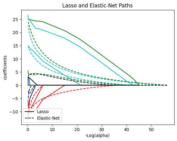
for coef_l, coef_e, c in zip(coefs_lasso, coefs_enet, colors):
    l1 = plt.plot(neg_log_alphas_lasso, coef_l, c=c)
    l2 = plt.plot(neg_log_alphas_enet, coef_e, linestyle="--", c=c)

plt.xlabel("-Log(alpha)")
plt.ylabel("coefficients")
plt.title("Lasso and Elastic-Net Paths")
plt.legend((l1[-1], l2[-1]), ("Lasso", "Elastic-Net"), loc="lower left")
plt.axis("tight")


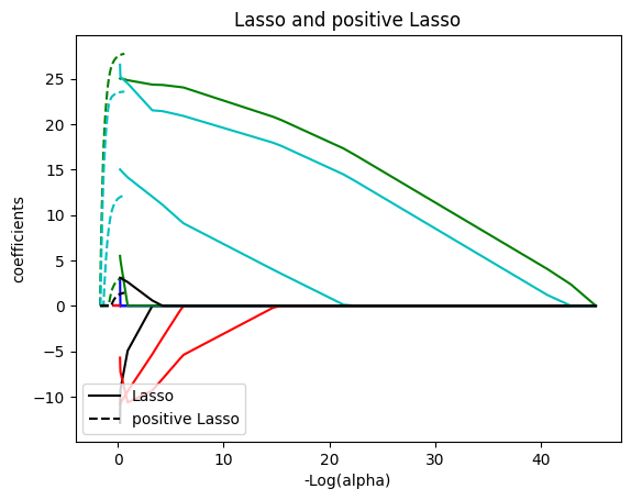
plt.figure(2)
neg_log_alphas_positive_lasso = -np.log10(alphas_positive_lasso)
for coef_l, coef_pl, c in zip(coefs_lasso, coefs_positive_lasso, colors):
    l1 = plt.plot(neg_log_alphas_lasso, coef_l, c=c)
    l2 = plt.plot(neg_log_alphas_positive_lasso, coef_pl, linestyle="--", c=c)

plt.xlabel("-Log(alpha)")
plt.ylabel("coefficients")
plt.title("Lasso and positive Lasso")
plt.legend((l1[-1], l2[-1]), ("Lasso", "positive Lasso"), loc="lower left")
plt.axis("tight")


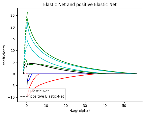
plt.figure(3)
neg_log_alphas_positive_enet = -np.log10(alphas_positive_enet)
for coef_e, coef_pe, c in zip(coefs_enet, coefs_positive_enet, colors):
    l1 = plt.plot(neg_log_alphas_enet, coef_e, c=c)
    l2 = plt.plot(neg_log_alphas_positive_enet, coef_pe, linestyle="--", c=c)

plt.xlabel("-Log(alpha)")
plt.ylabel("coefficients")
plt.title("Elastic-Net and positive Elastic-Net")
plt.legend((l1[-1], l2[-1]), ("Elastic-Net", "positive Elastic-Net"), loc="lower left")
plt.axis("tight")
plt.show()

Computing regularization path using the lasso...
Computing regularization path using the positive lasso...
Computing regularization path using the elastic net...
Computing regularization path using the positive elastic net...

../../_images/9c4dbcb8fc6d4e6e51b7cd6d1e33790bfe053aa2ea1f9bba76fe8fdce6b5db7d.png

../../_images/83dbcc232258c81a3de0edbf91f987ed6fae48812139ef8a55190948f196d33e.png

../../_images/5a96fee5cad22b3f250e3c90c096113ad98aa4ccdfdb827c7c9f750e8216fcdb.png

Introducción a métodos de regularización en Aprendizaje Automático

Contents

Introducción a métodos de regularización en Aprendizaje Automático#

Versión b.1#

Aprendizaje Automático [UCV]#

Plot de curva#

Resumen#

Definición: error \(\hat{e}\)#

Definición: Un problema general de optimización \(P(\lambda, s)\)#

Motivo#

Regresión lineal (OLS)#

Formulación de regresión lineal:#

Solución analítica (Ecuaciones normales)#

LASSO#

Forma lagrangeana:#

Forma con restricciones:#

Closed form solution#

Ridge regression#

Ridge: Formulación lagrangeana#

Solución analítica#

Laboratorio#

Generación de los datos#

Tarea#

Solution#

Generación del modelo#

Ordinary Least Squares#

Lasso: Formulación con restricciones#

Lasso: Formulación lagrangeana#

Ver resultados básicos#

Calculando el camino de regularización y los valores cuadráticos medios#

Métodos#

Mean Squared Error (MSE)#

Loss function#

Sección de gráficos#

Regularization path#

Mean Squared Error (MSE)#

Tarea#

Lasso con lagrangian formulation#

Solution (Lasso with constrained formulation)#

Selección de modelo: Eligiendo las mejores lambda y s#

Resumen de resultados#

Frameworks en producción (Real World)#

Usando Scikit-Learn#

Import library#

Attributes#

Methods#

Model selection via k-fold cross validation#

New Section#

Agregando columna al data frame de soluciones#

Comparando los valores de los coeficientes#

Regularization path per each fold#

Referencias#